Organizations often use Terraform Modules to orchestrate complex resource provisioning and provide a simple interface for developers to enter the required parameters to deploy the desired infrastructure. Modules enable code reuse and provide a method for organizations to standardize deployment of common workloads such as a three-tier web application, a cloud networking environment, or a data analytics pipeline. When building Terraform modules, it is common for the module author to start with manual testing. Manual testing is performed using commands such as terraform validate for syntax validation, terraform plan to preview the execution plan, and terraform apply followed by manual inspection of resource configuration in the AWS Management Console. Manual testing is prone to human error, not scalable, and can result in unintended issues. Because modules are used by multiple teams in the organization, it is important to ensure that any changes to the modules are extensively tested before the release. In this blog post, we will show you how to validate Terraform modules and how to automate the process using a Continuous Integration/Continuous Deployment (CI/CD) pipeline.
Terraform Test
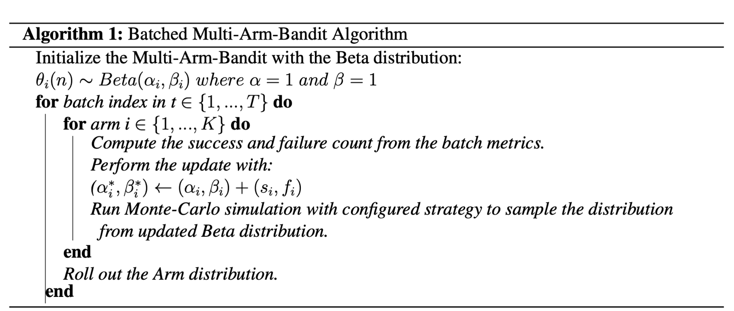
Terraform test is a new testing framework for module authors to perform unit and integration tests for Terraform modules. Terraform test can create infrastructure as declared in the module, run validation against the infrastructure, and destroy the test resources regardless if the test passes or fails. Terraform test will also provide warnings if there are any resources that cannot be destroyed. Terraform test uses the same HashiCorp Configuration Language (HCL) syntax used to write Terraform modules. This reduces the burden for modules authors to learn other tools or programming languages. Module authors run the tests using the command terraform test which is available on Terraform CLI version 1.6 or higher.
Module authors create test files with the extension *.tftest.hcl. These test files are placed in the root of the Terraform module or in a dedicated tests directory. The following elements are typically present in a Terraform tests file:
Provider block: optional, used to override the provider configuration, such as selecting AWS region where the tests run.
Variables block: the input variables passed into the module during the test, used to supply non-default values or to override default values for variables.
Run block: used to run a specific test scenario. There can be multiple run blocks per test file, Terraform executes run blocks in order. In each run block you specify the command Terraform (plan or apply), and the test assertions. Module authors can specify the conditions such as: length(var.items) != 0. A full list of condition expressions can be found in the HashiCorp documentation.
Terraform tests are performed in sequential order and at the end of the Terraform test execution, any failed assertions are displayed.
Basic test to validate resource creation
Now that we understand the basic anatomy of a Terraform tests file, let’s create basic tests to validate the functionality of the following Terraform configuration. This Terraform configuration will create an AWS CodeCommit repository with prefix name repo-.
Now we create a Terraform test file in the tests directory. See the following directory structure as an example:
├── main.tf
└── tests
└── basic.tftest.hcl
For this first test, we will not perform any assertion except for validating that Terraform execution plan runs successfully. In the tests file, we create a variable block to set the value for the variable repository_name. We also added the run block with command = plan to instruct Terraform test to run Terraform plan. The completed test should look like the following:
# basic.tftest.hcl

variables {
  repository_name = "MyRepo"
}

run "test_resource_creation" {
  command = plan
}
Now we will run this test locally. First ensure that you are authenticated into an AWS account, and run the terraform init command in the root directory of the Terraform module. After the provider is initialized, start the test using the terraform test command.
❯ terraform test
tests/basic.tftest.hcl... in progress
run "test_resource_creation"... pass
tests/basic.tftest.hcl... tearing down
tests/basic.tftest.hcl... pass
Our first test is complete, we have validated that the Terraform configuration is valid and the resource can be provisioned successfully. Next, let’s learn how to perform inspection of the resource state.
Create resource and validate resource name
Re-using the previous test file, we add the assertion block to checks if the CodeCommit repository name starts with a string repo- and provide error message if the condition fails. For the assertion, we use the startswith function. See the following example:
# basic.tftest.hcl

variables {
  repository_name = "MyRepo"
}

run "test_resource_creation" {
  command = plan

  assert {
    condition = startswith(aws_codecommit_repository.test.repository_name, "repo-")
    error_message = "CodeCommit repository name ${var.repository_name} did not start with the expected value of ‘repo-****’."
  }
}
Now, let’s assume that another module author made changes to the module by modifying the prefix from repo- to my-repo-. Here is the modified Terraform module.
We can catch this mistake by running the the terraform test command again.
❯ terraform test
tests/basic.tftest.hcl... in progress
run "test_resource_creation"... fail
╷
│ Error: Test assertion failed
│
│ on tests/basic.tftest.hcl line 9, in run "test_resource_creation":
│ 9: condition = startswith(aws_codecommit_repository.test.repository_name, "repo-")
│ ├────────────────
│ │ aws_codecommit_repository.test.repository_name is "my-repo-MyRepo"
│
│ CodeCommit repository name MyRepo did not start with the expected value 'repo-***'.
╵
tests/basic.tftest.hcl... tearing down
tests/basic.tftest.hcl... fail

Failure! 0 passed, 1 failed.
We have successfully created a unit test using assertions that validates the resource name matches the expected value. For more examples of using assertions see the Terraform Tests Docs. Before we proceed to the next section, don’t forget to fix the repository name in the module (revert the name back to repo- instead of my-repo-) and re-run your Terraform test.
Testing variable input validation
When developing Terraform modules, it is common to use variable validation as a contract test to validate any dependencies / restrictions. For example, AWS CodeCommit limits the repository name to 100 characters. A module author can use the length function to check the length of the input variable value. We are going to use Terraform test to ensure that the variable validation works effectively. First, we modify the module to use variable validation.
# main.tf

variable "repository_name" {
  type = string
  validation {
    condition = length(var.repository_name) <= 100
    error_message = "The repository name must be less than or equal to 100 characters."
  }
}

resource "aws_codecommit_repository" "test" {
  repository_name = format("repo-%s", var.repository_name)
  description = "Test repository."
}
By default, when variable validation fails during the execution of Terraform test, the Terraform test also fails. To simulate this, create a new test file and insert the repository_name variable with a value longer than 100 characters.
# var_validation.tftest.hcl

variables {
  repository_name = “this_is_a_repository_name_longer_than_100_characters_7rfD86rGwuqhF3TH9d3Y99r7vq6JZBZJkhw5h4eGEawBntZmvy”
}

run “test_invalid_var” {
  command = plan
}
Notice on this new test file, we also set the command to Terraform plan, why is that? Because variable validation runs prior to Terraform apply, thus we can save time and cost by skipping the entire resource provisioning. If we run this Terraform test, it will fail as expected.
❯ terraform test
tests/basic.tftest.hcl… in progress
run “test_resource_creation”… pass
tests/basic.tftest.hcl… tearing down
tests/basic.tftest.hcl… pass
tests/var_validation.tftest.hcl… in progress
run “test_invalid_var”… fail
╷
│ Error: Invalid value for variable
│
│ on main.tf line 1:
│ 1: variable “repository_name” {
│ ├────────────────
│ │ var.repository_name is “this_is_a_repository_name_longer_than_100_characters_7rfD86rGwuqhF3TH9d3Y99r7vq6JZBZJkhw5h4eGEawBntZmvy”
│
│ The repository name must be less than or equal to 100 characters.
│
│ This was checked by the validation rule at main.tf:3,3-13.
╵
tests/var_validation.tftest.hcl… tearing down
tests/var_validation.tftest.hcl… fail

Failure! 1 passed, 1 failed.
For other module authors who might iterate on the module, we need to ensure that the validation condition is correct and will catch any problems with input values. In other words, we expect the validation condition to fail with the wrong input. This is especially important when we want to incorporate the contract test in a CI/CD pipeline. To prevent our test from failing due introducing an intentional error in the test, we can use the expect_failures attribute. Here is the modified test file:
# var_validation.tftest.hcl

variables {
  repository_name = “this_is_a_repository_name_longer_than_100_characters_7rfD86rGwuqhF3TH9d3Y99r7vq6JZBZJkhw5h4eGEawBntZmvy”
}

run “test_invalid_var” {
  command = plan

  expect_failures = [
    var.repository_name
  ]
}
Now if we run the Terraform test, we will get a successful result.
❯ terraform test
tests/basic.tftest.hcl… in progress
run “test_resource_creation”… pass
tests/basic.tftest.hcl… tearing down
tests/basic.tftest.hcl… pass
tests/var_validation.tftest.hcl… in progress
run “test_invalid_var”… pass
tests/var_validation.tftest.hcl… tearing down
tests/var_validation.tftest.hcl… pass

Success! 2 passed, 0 failed.
As you can see, the expect_failures attribute is used to test negative paths (the inputs that would cause failures when passed into a module). Assertions tend to focus on positive paths (the ideal inputs). For an additional example of a test that validates functionality of a completed module with multiple interconnected resources, see this example in the Terraform CI/CD and Testing on AWS Workshop.
Orchestrating supporting resources
In practice, end-users utilize Terraform modules in conjunction with other supporting resources. For example, a CodeCommit repository is usually encrypted using an AWS Key Management Service (KMS) key. The KMS key is provided by end-users to the module using a variable called kms_key_id. To simulate this test, we need to orchestrate the creation of the KMS key outside of the module. In this section we will learn how to do that. First, update the Terraform module to add the optional variable for the KMS key.
# main.tf

variable "repository_name" {
  type = string
  validation {
    condition = length(var.repository_name) <= 100
    error_message = "The repository name must be less than or equal to 100 characters."
  }
}

variable "kms_key_id" {
  type = string
  default = ""
}

resource "aws_codecommit_repository" "test" {
  repository_name = format("repo-%s", var.repository_name)
  description = "Test repository."
  kms_key_id = var.kms_key_id != "" ? var.kms_key_id : null
}
In a Terraform test, you can instruct the run block to execute another helper module. The helper module is used by the test to create the supporting resources. We will create a sub-directory called setup under the tests directory with a single kms.tf file. We also create a new test file for KMS scenario. See the updated directory structure:
The new test will use two separate run blocks. The first run block (setup) executes the helper module to generate a KMS key. This is done by assigning the command apply which will run terraform apply to generate the KMS key. The second run block (codecommit_with_kms) will then use the KMS key ARN output of the first run as the input variable passed to the main module.
# with_kms.tftest.hcl

run "setup" {
  command = apply
  module {
    source = "./tests/setup"
  }
}

run "codecommit_with_kms" {
  command = apply

  variables {
    repository_name = "MyRepo"
    kms_key_id = run.setup.kms_key_id
  }

  assert {
    condition = aws_codecommit_repository.test.kms_key_id != null
    error_message = "KMS key ID attribute value is null"
  }
}
Go ahead and run the Terraform init, followed by Terraform test. You should get the successful result like below.
❯ terraform test
tests/basic.tftest.hcl... in progress
run "test_resource_creation"... pass
tests/basic.tftest.hcl... tearing down
tests/basic.tftest.hcl... pass
tests/var_validation.tftest.hcl... in progress
run "test_invalid_var"... pass
tests/var_validation.tftest.hcl... tearing down
tests/var_validation.tftest.hcl... pass
tests/with_kms.tftest.hcl... in progress
run "create_kms_key"... pass
run "codecommit_with_kms"... pass
tests/with_kms.tftest.hcl... tearing down
tests/with_kms.tftest.hcl... pass

Success! 4 passed, 0 failed.
We have learned how to run Terraform test and develop various test scenarios. In the next section we will see how to incorporate all the tests into a CI/CD pipeline.
Terraform Tests in CI/CD Pipelines
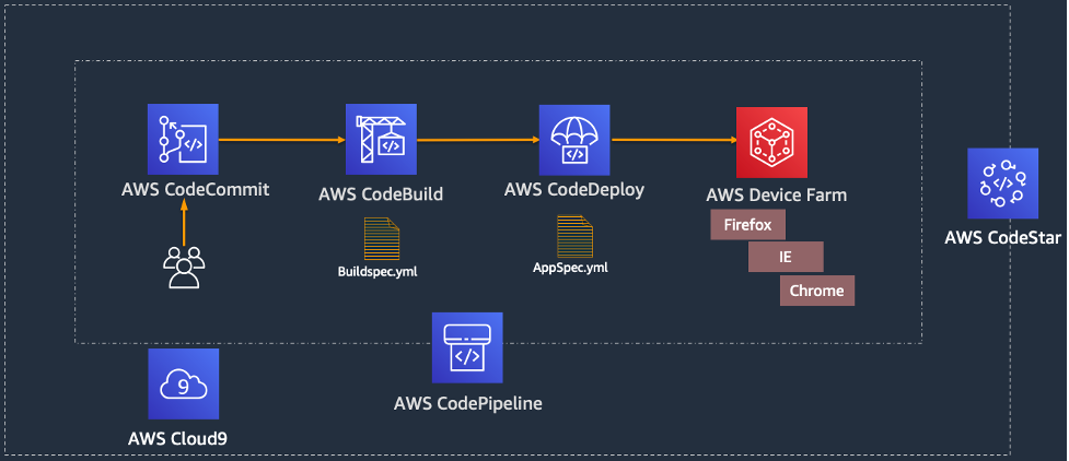
Now that we have seen how Terraform Test works locally, let’s see how the Terraform test can be leveraged to create a Terraform module validation pipeline on AWS. The following AWS services are used:
AWS CodeCommit – a secure, highly scalable, fully managed source control service that hosts private Git repositories.
AWS CodeBuild – a fully managed continuous integration service that compiles source code, runs tests, and produces ready-to-deploy software packages.
AWS CodePipeline – a fully managed continuous delivery service that helps you automate your release pipelines for fast and reliable application and infrastructure updates.
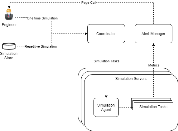
In the above architecture for a Terraform module validation pipeline, the following takes place:
A developer pushes Terraform module configuration files to a git repository (AWS CodeCommit).
AWS CodePipeline begins running the pipeline. The pipeline clones the git repo and stores the artifacts to an Amazon S3 bucket.
An AWS CodeBuild project configures a compute/build environment with Checkov installed from an image fetched from Docker Hub. CodePipeline passes the artifacts (Terraform module) and CodeBuild executes Checkov to run static analysis of the Terraform configuration files.
Another CodeBuild project configured with Terraform from an image fetched from Docker Hub. CodePipeline passes the artifacts (repo contents) and CodeBuild runs Terraform command to execute the tests.
CodeBuild uses a buildspec file to declare the build commands and relevant settings. Here is an example of the buildspec files for both CodeBuild Projects:
In the above buildspec, Checkov is run against the root directory of the cloned CodeCommit repository. This directory contains the configuration files for the Terraform module. Checkov also saves the output to a file named checkov.result.txt for further review or handling if needed. If Checkov fails, the pipeline will fail.
# Terraform Test
version: 0.1
phases:
  pre_build:
    commands:
      - terraform init
      - terraform validate

  build:
    commands:
      - terraform test
In the above buildspec, the terraform init and terraform validate commands are used to initialize Terraform, then check if the configuration is valid. Finally, the terraform test command is used to run the configured tests. If any of the Terraform tests fails, the pipeline will fail.
For a full example of the CI/CD pipeline configuration, please refer to the Terraform CI/CD and Testing on AWS workshop. The module validation pipeline mentioned above is meant as a starting point. In a production environment, you might want to customize it further by adding Checkov allow-list rules, linting, checks for Terraform docs, or pre-requisites such as building the code used in AWS Lambda.
Choosing various testing strategies
At this point you may be wondering when you should use Terraform tests or other tools such as Preconditions and Postconditions, Check blocks or policy as code. The answer depends on your test type and use-cases. Terraform test is suitable for unit tests, such as validating resources are created according to the naming specification. Variable validations and Pre/Post conditions are useful for contract tests of Terraform modules, for example by providing error warning when input variables value do not meet the specification. As shown in the previous section, you can also use Terraform test to ensure your contract tests are running properly. Terraform test is also suitable for integration tests where you need to create supporting resources to properly test the module functionality. Lastly, Check blocks are suitable for end to end tests where you want to validate the infrastructure state after all resources are generated, for example to test if a website is running after an S3 bucket configured for static web hosting is created.
When developing Terraform modules, you can run Terraform test in command = plan mode for unit and contract tests. This allows the unit and contract tests to run quicker and cheaper since there are no resources created. You should also consider the time and cost to execute Terraform test for complex / large Terraform configurations, especially if you have multiple test scenarios. Terraform test maintains one or many state files within the memory for each test file. Consider how to re-use the module’s state when appropriate. Terraform test also provides test mocking, which allows you to test your module without creating the real infrastructure.
Conclusion
In this post, you learned how to use Terraform test and develop various test scenarios. You also learned how to incorporate Terraform test in a CI/CD pipeline. Lastly, we also discussed various testing strategies for Terraform configurations and modules. For more information about Terraform test, we recommend the Terraform test documentation and tutorial. To get hands on practice building a Terraform module validation pipeline and Terraform deployment pipeline, check out the Terraform CI/CD and Testing on AWS Workshop.
Today, we’re excited to announce a new Workers Vitest integration – allowing you to write unit and integration tests via the popular testing framework, Vitest, that execute directly in our runtime, workerd!
This integration provides you with the ability to test anything related to your Worker!
For the first time, you can write unit tests that run within the same runtime that Cloudflare Workers run on in production, providing greater confidence that the behavior of your Worker in tests will be the same as when deployed to production. For integration tests, you can now write tests for Workers that are triggered by Cron Triggers in addition to traditional fetch() events. You can also more easily test complex applications that interact with KV, R2, D1, Queues, Service Bindings, and more Cloudflare products.
For all of your tests, you have access to Vitest features like snapshots, mocks, timers, and spies.
In addition to increased testing and functionality, you’ll also notice other developer experience improvements like hot-module-reloading, watch mode on by default, and per-test isolated storage. Meaning that, as you develop and edit your tests, they’ll automatically re-run, without you having to restart your test runner.
Get started testing Workers with Vitest
The easiest way to get started with testing your Workers via Vitest is to start a new Workers project via our create-cloudflare tool:
Running this command will scaffold a new project for you with the Workers Vitest integration already set up. An example unit test and integration test are also included.
Manual install and setup instructions
If you prefer to manually install and set up the Workers Vitest integration, begin by installing @cloudflare/vitest-pool-workers from npm:
@cloudflare/vitest-pool-workers has a peer dependency on a specific version of vitest. Modern versions of npm will install this automatically, but we recommend you install it explicitly too. Refer to the getting started guide for the current supported version. If you’re using TypeScript, add @cloudflare/vitest-pool-workers to your tsconfig.json’s types to get types for the cloudflare:test module:
@cloudflare/vitest-pool-workers has a peer dependency on a specific version of vitest. Modern versions of npm will install this automatically, but we recommend you install it explicitly too. Refer to the getting started guide for the current supported version. If you’re using TypeScript, add @cloudflare/vitest-pool-workers to your tsconfig.json’s types to get types for the cloudflare:test module:
With the new Workers Vitest Integration, you can test anything exported from your Worker in both unit and integration-style tests. Within these tests, you can also test connected resources like R2, KV, and Durable Objects, as well as applications involving multiple Workers.
Writing unit tests
In a Workers context, a unit test imports and directly calls functions from your Worker then asserts on their return values. Let’s say you have a Worker that looks like this:
export function add(a, b) {
  return a + b;
}

export default {
  async fetch(request) {
    const url = new URL(request.url);
    const a = parseInt(url.searchParams.get("a"));
    const b = parseInt(url.searchParams.get("b"));
    return new Response(add(a, b));
  }
}
After you’ve setup and installed the Workers Vitest integration, you can unit test this Worker by creating a new test file called index.spec.js with the following code:
Using the Workers Vitest integration, you can write unit tests like these for any of your Workers.
Writing integration tests
While unit tests are great for testing individual parts of your application, integration tests assess multiple units of functionality, ensuring that workflows and features work as expected. These are usually more complex than unit tests, but provide greater confidence that your app works as expected. In the Workers context, an integration test sends HTTP requests to your Worker and asserts on the HTTP responses.
With the Workers Vitest Integration, you can run integration tests by importing SELF from the new cloudflare:test utility like this:
// test/index.spec.ts
import { SELF } from "cloudflare:test";
import { it, expect } from "vitest";
import "../src";

// an integration test using SELF
it("sends request (integration style)", async () => {
   const response = await SELF.fetch("http://example.com/?a=3&b=4");
   expect(await response.text()).toMatchInlineSnapshot(`"7"`);
});
When using SELF for integration tests, your Worker code runs in the same context as the test runner. This means you can use mocks to control your Worker.
Testing different scenarios
Whether you’re writing unit or integration tests, if your application uses Cloudflare Developer Platform products (e.g. KV, R2, D1, Queues, or Durable Objects), you can test them. To demonstrate this, we have created a set of examples to help get you started testing.
Better testing experience === better testing
Having better testing tools makes it easier to test your projects right from the start, which leads to better overall quality and experience for your end users. The Workers Vitest integration provides that better experience, not just in terms of developer experience, but in making it easier to test your entire application.
The rest of this post will focus on how we built this new testing integration, diving into the internals of how Vitest works, the problems we encountered trying to get a framework to work within our runtime, and ultimately how we solved it and the improved DX that it unlocked.
How Vitest traditionally works
When you start Vitest’s CLI, it first collects and sequences all your test files. By default, Vitest uses a “threads” pool, which spawns Node.js worker threads for isolating and running tests in parallel. Each thread gets a test file to run, dynamically requesting and evaluating code as needed. When the test runner imports a module, it sends a request to the host’s “Vite Node Server” which will either return raw JavaScript code transformed by Vite, or an external module path. If raw code is returned, it will be executed using the node:vmrunInThisContext() function. If a module path is returned, it will be imported using dynamic import(). Transforming user code with Vite allows hot-module-reloading (HMR) — when a module changes, it’s invalidated in the module cache and a new version will be returned when it’s next imported.
Miniflare is a fully-local simulator for Cloudflare’s Developer Platform. Miniflare v2 provided a custom environment for Vitest that allowed you to run your tests inside the Workers sandbox. This meant you could import and call any function using Workers runtime APIs in your tests. You weren’t restricted to integration tests that just sent and received HTTP requests. In addition, this environment provided per-test isolated storage, automatically undoing any changes made at the end of each test. In Miniflare v2, this environment was relatively simple to implement. We’d already reimplemented Workers Runtime APIs in a Node.js environment, and could inject them using Vitest’s APIs into the global scope of the test runner.
By contrast, Miniflare v3 runs your Worker code inside the same workerd runtime that Cloudflare uses in production. Running tests directly in workerd presented a challenge — workerd runs in its own process, separate from the Node.js worker thread, and it’s not possible to reference JavaScript classes across a process boundary.
Solving the problem with custom pools
Instead, we use Vitest’s custom pools feature to run the test runner in Cloudflare Workers running locally with workerd. A pool receives test files to run and decides how to execute them. By executing the runner inside workerd, tests have direct access to Workers runtime APIs as they’re running in a Worker. WebSockets are used to send and receive serialisable RPC messages between the Node.js host and workerd process. Note we’re running the exact same test runner code originally designed for a Node-context inside a Worker here. This means our Worker needs to provide Node’s built-in modules, support for dynamic code evaluation, and loading of arbitrary modules from disk with Node-resolution behavior. The nodejs_compat compatibility flag provides support for some of Node’s built-in modules, but does not solve our other problems. For that, we had to get creative…
Dynamic code evaluation
For security reasons, the Cloudflare Workers runtime does not allow dynamic code evaluation via eval() or new Function(). It also requires all modules to be defined ahead-of-time before execution starts. The test runner doesn’t know what code to run until we start executing tests, so without lifting these restrictions, we have no way of executing the raw JavaScript code transformed by Vite nor importing arbitrary modules from disk. Fortunately, code that is only meant to run locally – like tests – has a much more relaxed security model than deployed code. To support local testing and other development-specific use-cases such as Vite’s new Runtime API, we added “unsafe-eval bindings” and “module-fallback services” to workerd.
Unsafe-eval bindings provide local-only access to the eval() function, and new Function()/new AsyncFunction()/new WebAssembly.Module() constructors. By exposing these through a binding, we retain control over which code has access to these features.
Using the unsafe-eval binding eval() method, we were able to implement a polyfill for the required vm.runInThisContext() function. While we could also implement loading of arbitrary modules from disk using unsafe-eval bindings, this would require us to rebuild workerd’s module resolution system in JavaScript. Instead, we allow workers to be configured with module fallback services. If enabled, imports that cannot be resolved by workerd become HTTP requests to the fallback service. These include the specifier, referrer, and whether it was an import or require. The service may respond with a module definition, or a redirect to another location if the resolved location doesn’t match the specifier. Requests originating from synchronous requires will block the main thread until the module is resolved. The Workers Vitest pool’s fallback service implements Node-like resolution with Node-style interoperability between CommonJS and ES modules.
Durable Objects as test runners
Now that we can run and import arbitrary code, the next step is to get Vitest’s thread worker running inside workerd. Every incoming request has its own request context. To improve overall performance, I/O objects such as streams, request/response bodies and WebSockets created in one request context cannot be used from another. This means if we want to use a WebSocket for RPC between the pool and our workerd processes, we need to make sure the WebSocket is only used from one request context. To coordinate this, we define a singleton Durable Object for accepting the RPC connection and running tests from. Functions using RPC such as resolving modules, reporting results and console logging will always use this singleton. We use Miniflare’s “magic proxy” system to get a reference to the singleton’s stub in Node.js, and send a WebSocket upgrade request directly to it. After adding a few more Node.js polyfills, and a basic cloudflare:test module to provide access to bindings and a function for creating ExecutionContexts, we’re able to write basic Workers unit tests! 🎉
Integration tests with hot-module-reloading
In addition to unit tests, we support integration testing with a special SELF service binding in the cloudflare:test module. This points to a special export default { fetch(...) {...} } handler which uses Vite to import your Worker’s main module.
Using Vite’s transformation pipeline here means your handler gets hot-module-reloading (HMR) for free! When code is updated, the module cache is invalidated, tests are rerun, and subsequent requests will execute with new code. The same approach of wrapping user code handlers applies to Durable Objects too, providing the same HMR benefits.
Integration tests can be written by calling SELF.fetch(), which will dispatch a fetch() event to your user code in the same global scope as your test, but under a different request context. This means global mocks apply to your Worker’s execution, as do request context lifetime restrictions. In particular, if you forget to call ctx.waitUntil(), you’ll see an appropriate error message. This wouldn’t be the case if you called your Worker’s handler directly in a unit test, as you’d be running under the runner singleton’s Durable Object request context, whose lifetime is automatically extended.
Most Workers applications will have at least one binding to a Cloudflare storage service, such as KV, R2 or D1. Ideally, tests should be self-contained and runnable in any order or on their own. To make this possible, writes to storage need to be undone at the end of each test, so reads by other tests aren’t affected. Whilst it’s possible to do this manually, it can be tricky to keep track of all writes and undo them in the correct order. For example, take the following two functions:
// helpers.ts
interface Env {
  NAMESPACE: KVNamespace;
}
// Get the current list stored in a KV namespace
export async function get(env: Env, key: string): Promise<string[]> {
  return await env.NAMESPACE.get(key, "json") ?? [];
}
// Add an item to the end of the list
export async function append(env: Env, key: string, item: string) {
  const value = await get(env, key);
  value.push(item);
  await env.NAMESPACE.put(key, JSON.stringify(value));
}
If we wanted to test these functions, we might write something like below. Note we have to keep track of all the keys we might write to, and restore their values at the end of tests, even if those tests fail.
// helpers.spec.ts
import { env } from "cloudflare:test";
import { beforeAll, beforeEach, afterEach, it, expect } from "vitest";
import { get, append } from "./helpers";

let startingList1: string | null;
let startingList2: string | null;
beforeEach(async () => {
  // Store values before each test
  startingList1 = await env.NAMESPACE.get("list 1");
  startingList2 = await env.NAMESPACE.get("list 2");
});
afterEach(async () => {
  // Restore starting values after each test
  if (startingList1 === null) {
    await env.NAMESPACE.delete("list 1");
  } else {
    await env.NAMESPACE.put("list 1", startingList1);
  }
  if (startingList2 === null) {
    await env.NAMESPACE.delete("list 2");
  } else {
    await env.NAMESPACE.put("list 2", startingList2);
  }
});

beforeAll(async () => {
  await append(env, "list 1", "one");
});

it("appends to one list", async () => {
  await append(env, "list 1", "two");
  expect(await get(env, "list 1")).toStrictEqual(["one", "two"]);
});

it("appends to two lists", async () => {
  await append(env, "list 1", "three");
  await append(env, "list 2", "four");
  expect(await get(env, "list 1")).toStrictEqual(["one", "three"]);
  expect(await get(env, "list 2")).toStrictEqual(["four"]);
});
This is slightly easier with the recently introduced onTestFinished() hook, but you still need to remember which keys were written to, or enumerate them at the start/end of tests. You’d also need to manage this for KV, R2, Durable Objects, caches and any other storage service you used. Ideally, the testing framework should just manage this all for you.
That’s exactly what the Workers Vitest pool does with the isolatedStorage option which is enabled by default. Any writes to storage performed in a test are automagically undone at the end of the test. To support seeding data in beforeAll() hooks, including those in nested describe()-blocks, a stack is used. Before each suite or test, a new frame is pushed to the storage stack. All writes performed by the test or associated beforeEach()/afterEach() hooks are written to the frame. After each suite or test, the top frame is popped from the storage stack, undoing any writes.
Miniflare implements simulators for storage services on top of Durable Objects with a separate blob store. When running locally, workerd uses SQLite for Durable Object storage. To implement isolated storage, we implement an on-disk stack of .sqlite database files by backing up the databases when “pushing”, and restoring backups when “popping”. Blobs stored in the separate store are retained through stack operations, and cleaned up at the end of each test run. Whilst this works, it involves copying lots of .sqlite files. Looking ahead, we’d like to explore using SQLite SAVEPOINTS for a more efficient solution.
Declarative request mocking
In addition to storage, most Workers will make outbound fetch() requests. For tests, it’s often useful to mock responses to these requests. Miniflare already allows you to specify an undiciMockAgent to route all requests through. The MockAgent class provides a declarative interface for specifying requests to mock and the corresponding responses to return. This API is relatively simple, whilst being flexible enough for advanced use cases. We provide an instance of MockAgent as fetchMock in the cloudflare:test module.
import { fetchMock } from "cloudflare:test";
import { beforeAll, afterEach, it, expect } from "vitest";

beforeAll(() => {
  // Enable outbound request mocking...
  fetchMock.activate();
  // ...and throw errors if an outbound request isn't mocked
  fetchMock.disableNetConnect();
});
// Ensure we matched every mock we defined
afterEach(() => fetchMock.assertNoPendingInterceptors());

it("mocks requests", async () => {
  // Mock the first request to `https://example.com`
  fetchMock
    .get("https://example.com")
    .intercept({ path: "/" })
    .reply(200, "body");

  const response = await fetch("https://example.com/");
  expect(await response.text()).toBe("body");
});
To implement this, we bundled a stripped down version of undici containing just the MockAgent code. We then built a custom undiciDispatcher that used the Worker’s global fetch() function instead of undici’s built-in HTTP implementation based on llhttp and node:net.
Testing Durable Objects directly
Finally, Miniflare v2’s custom Vitest environment provided support for accessing the instance methods and state of Durable Objects in tests directly. This allowed you to unit test Durable Objects like any other JavaScript class—you could mock particular methods and properties, or immediately call specific handlers like alarm(). To implement this in workerd, we rely on our existing wrapping of user Durable Objects for Vite transforms and hot-module reloading. When you call the runInDurableObject(stub, callback) function from cloudflare:test, we store callback in a global cache and send a special fetch() request to stub which is intercepted by the wrapper. The wrapper executes the callback in the request context of the Durable Object, and stores the result in the same cache. runInDurableObject() then reads from this cache, and returns the result.
Note that this assumes the Durable Object is running in the same isolate as the runInDurableObject() call. While this is true for same-Worker Durable Objects running locally, it means Durable Objects defined in auxiliary workers can’t be accessed directly.
Try it out!
We are excited to release the @cloudflare/vitest-pool-workers package on npm, and to provide an improved testing experience for you.
Make sure to read the Write your first test guide and begin writing unit and integration tests today! If you’ve been writing tests using one of our previous options, our unstable_devmigration guide or our Miniflare 2 migration guide should explain key differences and help you move your tests over quickly.
If you run into issues or have suggestions for improvements, please file an issue in our GitHub repo or reach out via our Developer Discord.
In this post, we’re excited to introduce SafeTest, a revolutionary library that offers a fresh perspective on End-To-End (E2E) tests for web-based User Interface (UI) applications.
The Challenges of Traditional UI Testing
Traditionally, UI tests have been conducted through either unit testing or integration testing (also referred to as End-To-End (E2E) testing). However, each of these methods presents a unique trade-off: you have to choose between controlling the test fixture and setup, or controlling the test driver.
For instance, when using react-testing-library, a unit testing solution, you maintain complete control over what to render and how the underlying services and imports should behave. However, you lose the ability to interact with an actual page, which can lead to a myriad of pain points:
Difficulty in interacting with complex UI elements like <Dropdown /> components.
Inability to test CORS setup or GraphQL calls.
Lack of visibility into z-index issues affecting click-ability of buttons.
Complex and unintuitive authoring and debugging of tests.
Conversely, using integration testing tools like Cypress or Playwright provides control over the page, but sacrifices the ability to instrument the bootstrapping code for the app. These tools operate by remotely controlling a browser to visit a URL and interact with the page. This approach has its own set of challenges:
Difficulty in making calls to an alternative API endpoint without implementing custom network layer API rewrite rules.
Inability to make assertions on spies/mocks or execute code within the app.
Testing something like dark mode entails clicking the theme switcher or knowing the localStorage mechanism to override.
Inability to test segments of the app, for example if a component is only visible after clicking a button and waiting for a 60 second timer to countdown, the test will need to run those actions and will be at least a minute long.
Recognizing these challenges, solutions like E2E Component Testing have emerged, with offerings from Cypress and Playwright. While these tools attempt to rectify the shortcomings of traditional integration testing methods, they have other limitations due to their architecture. They start a dev server with bootstrapping code to load the component and/or setup code you want, which limits their ability to handle complex enterprise applications that might have OAuth or a complex build pipeline. Moreover, updating TypeScript usage could break your tests until the Cypress/Playwright team updates their runner.
Welcome to SafeTest
SafeTest aims to address these issues with a novel approach to UI testing. The main idea is to have a snippet of code in our application bootstrapping stage that injects hooks to run our tests (see the How Safetest Works sections for more info on what this is doing). Note that how this works has no measurable impact on the regular usage of your app since SafeTest leverages lazy loading to dynamically load the tests only when running the tests (in the README example, the tests aren’t in the production bundle at all). Once that’s in place, we can use Playwright to run regular tests, thereby achieving the ideal browser control we want for our tests.
This approach also unlocks some exciting features:
Deep linking to a specific test without needing to run a node test server.
Two-way communication between the browser and test (node) context.
Access to all the DX features that come with Playwright (excluding the ones that come with @playwright/test).
Video recording of tests, trace viewing, and pause page functionality for trying out different page selectors/actions.
Ability to make assertions on spies in the browser in node, matching snapshot of the call within the browser.
Test Examples with SafeTest
SafeTest is designed to feel familiar to anyone who has conducted UI tests before, as it leverages the best parts of existing solutions. Here’s an example of how to test an entire application:
import { describe, it, expect } from 'safetest/jest';
import { render } from 'safetest/react';

describe('my app', () => {
  it('loads the main page', async () => {
    const { page } = await render();

    await expect(page.getByText('Welcome to the app')).toBeVisible();
    expect(await page.screenshot()).toMatchImageSnapshot();
  });
});
We can just as easily test a specific component
import { describe, it, expect, browserMock } from 'safetest/jest'; import { render } from 'safetest/react';
SafeTest utilizes React Context to allow for value overrides during tests. For an example of how this works, let’s assume we have a fetchPeople function used in a component:
import { useAsync } from 'react-use'; import { fetchPerson } from './api/person';
The render function also accepts a function that will be passed the initial app component, allowing for the injection of any desired elements anywhere in the app:
With overrides, we can write complex test cases such as ensuring a service method which combines API requests from /foo, /bar, and /baz, has the correct retry mechanism for just the failed API requests and still maps the return value correctly. So if /bar takes 3 attempts to resolve the method will make a total of 5 API calls.
Overrides aren’t limited to just API calls (since we can use also use page.route), we can also override specific app level values like feature flags or changing some static value:
+const Language = createOverride(navigator.language); export const LanguageChanger = () => { - const language = navigator.language; + const language = Language.useValue(); return <div>Current language is { language } </div>; }
await expect(page.getByText('Current language is abc')).toBeVisible(); }); });
Overrides are a powerful feature of SafeTest and the examples here only scratch the surface. For more information and examples, refer to the Overrides section on the README.
Many large corporations need a form of authentication to use the app. Typically, navigating to localhost:3000 just results in a perpetually loading page. You need to go to a different port, like localhost:8000, which has a proxy server to check and/or inject auth credentials into underlying service calls. This limitation is one of the main reasons that Cypress/Playwright Component Tests aren’t suitable for use at Netflix.
However, there’s usually a service that can generate test users whose credentials we can use to log in and interact with the application. This facilitates creating a light wrapper around SafeTest to automatically generate and assume that test user. For instance, here’s basically how we do it at Netflix:
import { setup } from 'safetest/setup'; import { createTestUser, addCookies } from 'netflix-test-helper';
type Setup = Parameters<typeof setup>[0] & { extraUserOptions?: UserOptions; };
After setting this up, we simply import the above package in place of where we would have used safetest/setup.
Beyond React
While this post focused on how SafeTest works with React, it’s not limited to just React. SafeTest also works with Vue, Svelte, Angular, and even can run on NextJS or Gatsby. It also runs using either Jest or Vitest based on which test runner your scaffolding started you off with. The examples folder demonstrates how to use SafeTest with different tooling combinations, and we encourage contributions to add more cases.
At its core, SafeTest is an intelligent glue for a test runner, a UI library, and a browser runner. Though the most common usage at Netflix employs Jest/React/Playwright, it’s easy to add more adapters for other options.
Conclusion
SafeTest is a powerful testing framework that’s being adopted within Netflix. It allows for easy authoring of tests and provides comprehensive reports when and how any failures occurred, complete with links to view a playback video or manually run the test steps to see what broke. We’re excited to see how it will revolutionize UI testing and look forward to your feedback and contributions.
Internet connections are most often marketed and sold on the basis of "speed", with providers touting the number of megabits or gigabits per second that their various service tiers are supposed to provide. This marketing has largely been successful, as most subscribers believe that "more is better”. Furthermore, many national broadband plans in countries around the world include specific target connection speeds. However, even with a high speed connection, gamers may encounter sluggish performance, while video conference participants may experience frozen video or audio dropouts. Speeds alone don't tell the whole story when it comes to Internet connection quality.
Additional factors like latency, jitter, and packet loss can significantly impact end user experience, potentially leading to situations where higher speed connections actually deliver a worse user experience than lower speed connections. Connection performance and quality can also vary based on usage – measured average speed will differ from peak available capacity, and latency varies under loaded and idle conditions.
The new Cloudflare Radar Internet Quality page
A little more than three years ago, as residential Internet connections were strained because of the shift towards working and learning from home due to the COVID-19 pandemic, Cloudflare announced the speed.cloudflare.com speed test tool, which enabled users to test the performance and quality of their Internet connection. Within the tool, users can download the results of their individual test as a CSV, or share the results on social media. However, there was no aggregated insight into Cloudflare speed test results at a network or country level to provide a perspective on connectivity characteristics across a larger population.
Today, we are launching these long-missing aggregated connection performance and quality insights on Cloudflare Radar. The new Internet Quality page provides both country and network (autonomous system) level insight into Internet connection performance (bandwidth) and quality (latency, jitter) over time. (Your Internet service provider is likely an autonomous system with its own autonomous system number (ASN), and many large companies, online platforms, and educational institutions also have their own autonomous systems and associated ASNs.) The insights we are providing are presented across two sections: the Internet Quality Index (IQI), which estimates average Internet quality based on aggregated measurements against a set of Cloudflare & third-party targets, and Connection Quality, which presents peak/best case connection characteristics based on speed.cloudflare.com test results aggregated over the previous 90 days. (Details on our approach to the analysis of this data are presented below.)
Users may note that individual speed test results, as well as the aggregate speed test results presented on the Internet Quality page will likely differ from those presented by other speed test tools. This can be due to a number of factors including differences in test endpoint locations (considering both geographic and network distance), test content selection, the impact of “rate boosting” by some ISPs, and testing over a single connection vs. multiple parallel connections. Infrequent testing (on any speed test tool) by users seeking to confirm perceived poor performance or validate purchased speeds will also contribute to the differences seen in the results published by the various speed test platforms.
And as we announced in April, Cloudflare has partnered with Measurement Lab (M-Lab) to create a publicly-available, queryable repository for speed test results. M-Lab is a non-profit third-party organization dedicated to providing a representative picture of Internet quality around the world. M-Lab produces and hosts the Network Diagnostic Tool, which is a very popular network quality test that records millions of samples a day. Given their mission to provide a publicly viewable, representative picture of Internet quality, we chose to partner with them to provide an accurate view of your Internet experience and the experience of others around the world using openly available data.
Connection speed & quality data is important
While most advertisements for fixed broadband and mobile connectivity tend to focus on download speeds (and peak speeds at that), there’s more to an Internet connection, and the user’s experience with that Internet connection, than that single metric. In addition to download speeds, users should also understand the upload speeds that their connection is capable of, as well as the quality of the connection, as expressed through metrics known as latency and jitter. Getting insight into all of these metrics provides a more well-rounded view of a given Internet connection, or in aggregate, the state of Internet connectivity across a geography or network.
The concept of download speeds are fairly well understood as a measure of performance. However, it is important to note that the average download speeds experienced by a user during common Web browsing activities, which often involves the parallel retrieval of multiple smaller files from multiple hosts, can differ significantly from peak download speeds, where the user is downloading a single large file (such as a video or software update), which allows the connection to reach maximum performance. The bandwidth (speed) available for upload is sometimes mentioned in ISP advertisements, but doesn’t receive much attention. (And depending on the type of Internet connection, there’s often a significant difference between the available upload and download speeds.) However, the importance of upload came to the forefront in 2020 as video conferencing tools saw a surge in usage as both work meetings and school classes shifted to the Internet during the COVID-19 pandemic. To share your audio and video with other participants, you need sufficient upload bandwidth, and this issue was often compounded by multiple people sharing a single residential Internet connection.
Latency is the time it takes data to move through the Internet, and is measured in the number of milliseconds that it takes a packet of data to go from a client (such as your computer or mobile device) to a server, and then back to the client. In contrast to speed metrics, lower latency is preferable. This is especially true for use cases like online gaming where latency can make a difference between a character’s life and death in the game, as well as video conferencing, where higher latency can cause choppy audio and video experiences, but it also impacts web page performance. The latency metric can be further broken down into loaded and idle latency. The former measures latency on a loaded connection, where bandwidth is actively being consumed, while the latter measures latency on an “idle” connection, when there is no other network traffic present. (These specific loaded and idle definitions are from the device’s perspective, and more specifically, from the speed test application’s perspective. Unless the speed test is being performed directly from a router, the device/application doesn't have insight into traffic on the rest of the network.) Jitter is the average variation found in consecutive latency measurements, and can be measured on both idle and loaded connections. A lower number means that the latency measurements are more consistent. As with latency, Internet connections should have minimal jitter, which helps provide more consistent performance.
Our approach to data analysis
The Internet Quality Index (IQI) and Connection Quality sections get their data from two different sources, providing two different (albeit related) perspectives. Under the hood they share some common principles, though.
IQI builds upon the mechanism we already use to regularly benchmark ourselves against other industry players. It is based on end user measurements against a set of Cloudflare and third-party targets, meant to represent a pattern that has become very common in the modern Internet, where most content is served from distribution networks with points of presence spread throughout the world. For this reason, and by design, IQI will show worse results for regions and Internet providers that rely on international (rather than peering) links for most content.
IQI is also designed to reflect the traffic load most commonly associated with web browsing, rather than more intensive use. This, and the chosen set of measurement targets, effectively biases the numbers towards what end users experience in practice (where latency plays an important role in how fast things can go).
For each metric covered by IQI, and for each ASN, we calculate the 25th percentile, median, and 75th percentile at 15 minute intervals. At the country level and above, the three calculated numbers for each ASN visible from that region are independently aggregated. This aggregation takes the estimated user population of each ASN into account, biasing the numbers away from networks that source a lot of automated traffic but have few end users.
The Connection Quality section gets its data from the Cloudflare Speed Test tool, which exercises a user's connection in order to see how well it is able to perform. It measures against the closest Cloudflare location, providing a good balance of realistic results and network proximity to the end user. We have a presence in 285 cities around the world, allowing us to be pretty close to most users.
Similar to the IQI, we calculate the 25th percentile, median, and 75th percentile for each ASN. But here these three numbers are immediately combined using an operation called the trimean — a single number meant to balance the best connection quality that most users have, with the best quality available from that ASN (users may not subscribe to the best available plan for a number of reasons).
Because users may choose to run a speed test for different motives at different times, and also because we take privacy very seriously and don’t record any personally identifiable information along with test results, we aggregate at 90-day intervals to capture as much variability as we can.
At the country level and above, the calculated trimean for each ASN in that region is aggregated. This, again, takes the estimated user population of each ASN into account, biasing the numbers away from networks that have few end users but which may still have technicians using the Cloudflare Speed Test to assess the performance of their network.
Navigating the Internet Quality page
The new Internet Quality page includes three views: Global, country-level, and autonomous system (AS). In line with the other pages on Cloudflare Radar, the country-level and AS pages show the same data sets, differing only in their level of aggregation. Below, we highlight the various components of the Internet Quality page.
Global
The top section of the global (worldwide) view includes time series graphs of the Internet Quality Index metrics aggregated at a continent level. The time frame shown in the graphs is governed by the selection made in the time frame drop down at the upper right of the page, and at launch, data for only the last three months is available. For users interested in examining a specific continent, clicking on the other continent names in the legend removes them from the graph. Although continent-level aggregation is still rather coarse, it still provides some insight into regional Internet quality around the world.
Further down the page, the Connection Quality section presents a choropleth map, with countries shaded according to the values of the speed, latency, or jitter metric selected from the drop-down menu. Hovering over a country displays a label with the country’s name and metric value, and clicking on the country takes you to the country’s Internet Quality page. Note that in contrast to the IQI section, the Connection Quality section always displays data aggregated over the previous 90 days.
Country-level
Within the country-level page (using Canada as an example in the figures below), the country’s IQI metrics over the selected time frame are displayed. These time series graphs show the median bandwidth, latency, and DNS response time within a shaded band bounded at the 25th and 75th percentile and represent the average expected user experience across the country, as discussed in the Our approach to data analysis section above.
Below that is the Connection Quality section, which provides a summary view of the country’s measured upload and download speeds, as well as latency and jitter, over the previous 90 days. The colored wedges in the Performance Summary graph are intended to illustrate aggregate connection quality at a glance, with an “ideal” connection having larger upload and download wedges and smaller latency and jitter wedges. Hovering over the wedges displays the metric’s value, which is also shown in the table to the right of the graph.
Below that, the Bandwidth and Latency/Jitter histograms illustrate the bucketed distribution of upload and download speeds, and latency and jitter measurements. In some cases, the speed histograms may show a noticeable bar at 1 Gbps, or 1000 ms (1 second) on the latency/jitter histograms. The presence of such a bar indicates that there is a set of measurements with values greater than the 1 Gbps/1000 ms maximum histogram values.
Autonomous system level
Within the upper-right section of the country-level page, a list of the top five autonomous systems within the country is shown. Clicking on an ASN takes you to the Performance page for that autonomous system. For others not displayed in the top five list, you can use the search bar at the top of the page to search by autonomous system name or number. The graphs shown within the AS level view are identical to those shown at a country level, but obviously at a different level of aggregation. You can find the ASN that you are connected to from the My Connection page on Cloudflare Radar.
Exploring connection performance & quality data
Digging into the IQI and Connection Quality visualizations can surface some interesting observations, including characterizing Internet connections, and the impact of Internet disruptions, including shutdowns and network issues. We explore some examples below.
Characterizing Internet connections
Verizon FiOS is a residential fiber-based Internet service available to customers in the United States. Fiber-based Internet services (as opposed to cable-based, DSL, dial-up, or satellite) will generally offer symmetric upload and download speeds, and the FiOS plans page shows this to be the case, offering 300 Mbps (upload & download), 500 Mbps (upload & download), and “1 Gig” (Verizon claims average wired speeds between 750-940 Mbps download / 750-880 Mbps upload) plans. Verizon carries FiOS traffic on AS701 (labeled UUNET due to a historical acquisition), and in looking at the bandwidth histogram for AS701, several things stand out. The first is a rough symmetry in upload and download speeds. (A cable-based Internet service provider, in contrast, would generally show a wide spread of download speeds, but have upload speeds clustered at the lower end of the range.) Another is the peaks around 300 Mbps and 750 Mbps, suggesting that the 300 Mbps and “1 Gig” plans may be more popular than the 500 Mbps plan. It is also clear that there are a significant number of test results with speeds below 300 Mbps. This is due to several factors: one is that Verizon also carries lower speed non-FiOS traffic on AS701, while another is that erratic nature of in-home WiFi often means that the speeds achieved on a test will be lower than the purchased service level.
Traffic shifts drive latency shifts
On May 9, 2023, the government of Pakistan ordered the shutdown of mobile network services in the wake of protests following the arrest of former Prime Minister Imran Khan. Our blog post covering this shutdown looked at the impact from a traffic perspective. Within the post, we noted that autonomous systems associated with fixed broadband networks saw significant increases in traffic when the mobile networks were shut down – that is, some users shifted to using fixed networks (home broadband) when mobile networks were unavailable.
Examining IQI data after the blog post was published, we found that the impact of this traffic shift was also visible in our latency data. As can be seen in the shaded area of the graph below, the shutdown of the mobile networks resulted in the median latency dropping about 25% as usage shifted from higher latency mobile networks to lower latency fixed broadband networks. An increase in latency is visible in the graph when mobile connectivity was restored on May 12.
Bandwidth shifts as a potential early warning sign
On April 4, UK mobile operator Virgin Media suffered several brief outages. In examining the IQI bandwidth graph for AS5089, the ASN used by Virgin Media (formerly branded as NTL), indications of a potential problem are visible several days before the outages occurred, as median bandwidth dropped by about a third, from around 35 Mbps to around 23 Mbps. The outages are visible in the circled area in the graph below. Published reports indicate that the problems lasted into April 5, in line with the lower median bandwidth measured through mid-day.
Submarine cable issues cause slower browsing
On June 5, Philippine Internet provider PLDTTweeted an advisory that noted “One of our submarine cable partners confirms a loss in some of its internet bandwidth capacity, and thus causing slower Internet browsing.” IQI latency and bandwidth graphs for AS9299, a primary ASN used by PLDT, shows clear shifts starting around 06:45 UTC (14:45 local time). Median bandwidth dropped by half, from 17 Mbps to 8 Mbps, while median latency increased by 75% from 37 ms to around 65 ms. 75th percentile latency also saw a significant increase, nearly tripling from 63 ms to 180 ms coincident with the reported submarine cable issue.
Conclusion
Making network performance and quality insights available on Cloudflare Radar supports Cloudflare’s mission to help build a better Internet. However, we’re not done yet – we have more enhancements planned. These include making data available at a more granular geographical level (such as state and possibly city), incorporating AIM scores to help assess Internet quality for specific types of use cases, and embedding the Cloudflare speed test directly on Radar using the open source JavaScript module.
In the meantime, we invite you to use speed.cloudflare.com to test the performance and quality of your Internet connection, share any country or AS-level insights you discover on social media (tag @CloudflareRadar on Twitter or @[email protected] on Mastodon), and explore the underlying data through the M-Lab repository or the Radar API.
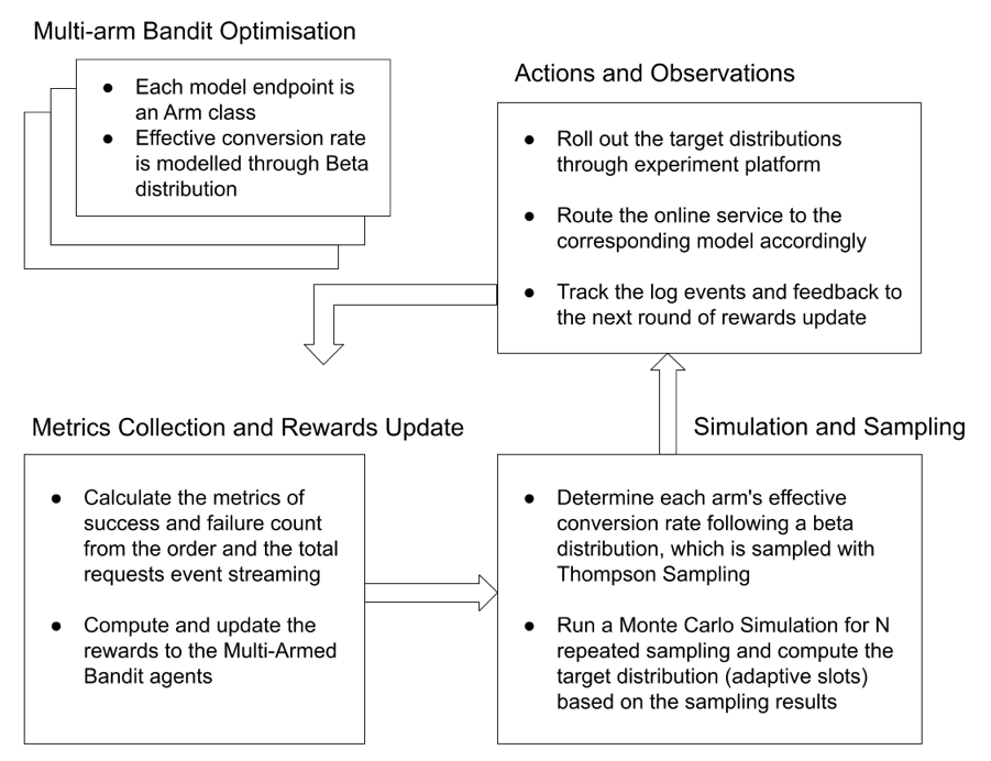
Picture yourself enthralled by the latest episode of your beloved Netflix series, delighting in an uninterrupted, high-definition streaming experience. Behind these perfect moments of entertainment is a complex mechanism, with numerous gears and cogs working in harmony. But what happens when this machinery needs a transformation? This is where large-scale system migrations come into play. Our previous blog post presented replay traffic testing — a crucial instrument in our toolkit that allows us to implement these transformations with precision and reliability.
Replay traffic testing gives us the initial foundation of validation, but as our migration process unfolds, we are met with the need for a carefully controlled migration process. A process that doesn’t just minimize risk, but also facilitates a continuous evaluation of the rollout’s impact. This blog post will delve into the techniques leveraged at Netflix to introduce these changes to production.
Sticky Canaries
Canary deployments are an effective mechanism for validating changes to a production backend service in a controlled and limited manner, thus mitigating the risk of unforeseen consequences that may arise due to the change. This process involves creating two new clusters for the updated service; a baseline cluster containing the current version running in production and a canary cluster containing the new version of the service. A small percentage of production traffic is redirected to the two new clusters, allowing us to monitor the new version’s performance and compare it against the current version. By collecting and analyzing key performance metrics of the service over time, we can assess the impact of the new changes and determine if they meet the availability, latency, and performance requirements.
Some product features require a lifecycle of requests between the customer device and a set of backend services to drive the feature. For instance, video playback functionality on Netflix involves requesting URLs for the streams from a service, calling the CDN to download the bits from the streams, requesting a license to decrypt the streams from a separate service, and sending telemetry indicating the successful start of playback to yet another service. By tracking metrics only at the level of service being updated, we might miss capturing deviations in broader end-to-end system functionality.
Sticky Canary is an improvement to the traditional canary process that addresses this limitation. In this variation, the canary framework creates a pool of unique customer devices and then routes traffic for this pool consistently to the canary and baseline clusters for the duration of the experiment. Apart from measuring service-level metrics, the canary framework is able to keep track of broader system operational and customer metrics across the canary pool and thereby detect regressions on the entire request lifecycle flow.
Sticky Canary
It is important to note that with sticky canaries, devices in the canary pool continue to be routed to the canary throughout the experiment, potentially resulting in undesirable behavior persisting through retries on customer devices. Therefore, the canary framework is designed to monitor operational and customer KPI metrics to detect persistent deviations and terminate the canary experiment if necessary.
Canaries and sticky canaries are valuable tools in the system migration process. Compared to replay testing, canaries allow us to extend the validation scope beyond the service level. They enable verification of the broader end-to-end system functionality across the request lifecycle for that functionality, giving us confidence that the migration will not cause any disruptions to the customer experience. Canaries also provide an opportunity to measure system performance under different load conditions, allowing us to identify and resolve any performance bottlenecks. They enable us to further fine-tune and configure the system, ensuring the new changes are integrated smoothly and seamlessly.
A/B Testing
A/B testing is a widely recognized method for verifying hypotheses through a controlled experiment. It involves dividing a portion of the population into two or more groups, each receiving a different treatment. The results are then evaluated using specific metrics to determine whether the hypothesis is valid. The industry frequently employs the technique to assess hypotheses related to product evolution and user interaction. It is also widely utilized at Netflix to test changes to product behavior and customer experience.
A/B testing is also a valuable tool for assessing significant changes to backend systems. We can determine A/B test membership in either device application or backend code and selectively invoke new code paths and services. Within the context of migrations, A/B testing enables us to limit exposure to the migrated system by enabling the new path for a smaller percentage of the member base. Thereby controlling the risk of unexpected behavior resulting from the new changes. A/B testing is also a key technique in migrations where the updates to the architecture involve changing device contracts as well.
Canary experiments are typically conducted over periods ranging from hours to days. However, in certain instances, migration-related experiments may be required to span weeks or months to obtain a more accurate understanding of the impact on specific Quality of Experience (QoE) metrics. Additionally, in-depth analyses of particular business Key Performance Indicators (KPIs) may require longer experiments. For instance, envision a migration scenario where we enhance the playback quality, anticipating that this improvement will lead to more customers engaging with the play button. Assessing relevant metrics across a considerable sample size is crucial for obtaining a reliable and confident evaluation of the hypothesis. A/B frameworks work as effective tools to accommodate this next step in the confidence-building process.
In addition to supporting extended durations, A/B testing frameworks offer other supplementary capabilities. This approach enables test allocation restrictions based on factors such as geography, device platforms, and device versions, while also allowing for analysis of migration metrics across similar dimensions. This ensures that the changes do not disproportionately impact specific customer segments. A/B testing also provides adaptability, permitting adjustments to allocation size throughout the experiment.
We might not use A/B testing for every backend migration. Instead, we use it for migrations in which changes are expected to impact device QoE or business KPIs significantly. For example, as discussed earlier, if the planned changes are expected to improve client QoE metrics, we would test the hypothesis via A/B testing.
Dialing Traffic
After completing the various stages of validation, such as replay testing, sticky canaries, and A/B tests, we can confidently assert that the planned changes will not significantly impact SLAs (service-level-agreement), device level QoE, or business KPIs. However, it is imperative that the final rollout is regulated to ensure that any unnoticed and unexpected problems do not disrupt the customer experience. To this end, we have implemented traffic dialing as the last step in mitigating the risk associated with enabling the changes in production.
A dial is a software construct that enables the controlled flow of traffic within a system. This construct samples inbound requests using a distribution function and determines whether they should be routed to the new path or kept on the existing path. The decision-making process involves assessing whether the distribution function’s output aligns within the range of the predefined target percentage. The sampling is done consistently using a fixed parameter associated with the request. The target percentage is controlled via a globally scoped dynamic property that can be updated in real-time. By increasing or decreasing the target percentage, traffic flow to the new path can be regulated instantaneously.
Dial
The selection of the actual sampling parameter depends on the specific migration requirements. A dial can be used to randomly sample all requests, which is achieved by selecting a variable parameter like a timestamp or a random number. Alternatively, in scenarios where the system path must remain constant with respect to customer devices, a constant device attribute such as deviceId is selected as the sampling parameter. Dials can be applied in several places, such as device application code, the relevant server component, or even at the API gateway for edge API systems, making them a versatile tool for managing migrations in complex systems.
Traffic is dialed over to the new system in measured discrete steps. At every step, relevant stakeholders are informed, and key metrics are monitored, including service, device, operational, and business metrics. If we discover an unexpected issue or notice metrics trending in an undesired direction during the migration, the dial gives us the capability to quickly roll back the traffic to the old path and address the issue.
The dialing steps can also be scoped at the data center level if traffic is served from multiple data centers. We can start by dialing traffic in a single data center to allow for an easier side-by-side comparison of key metrics across data centers, thereby making it easier to observe any deviations in the metrics. The duration of how long we run the actual discrete dialing steps can also be adjusted. Running the dialing steps for longer periods increases the probability of surfacing issues that may only affect a small group of members or devices and might have been too low to capture and perform shadow traffic analysis. We can complete the final step of migrating all the production traffic to the new system using the combination of gradual step-wise dialing and monitoring.
Migrating Persistent Stores
Stateful APIs pose unique challenges that require different strategies. While the replay testing technique discussed in the previous part of this blog series can be employed, additional measures outlined earlier are necessary.
This alternate migration strategy has proven effective for our systems that meet certain criteria. Specifically, our data model is simple, self-contained, and immutable, with no relational aspects. Our system doesn’t require strict consistency guarantees and does not use database transactions. We adopt an ETL-based dual-write strategy that roughly follows this sequence of steps:
Initial Load through an ETL process: Data is extracted from the source data store, transformed into the new model, and written to the newer data store through an offline job. We use custom queries to verify the completeness of the migrated records.
Continuous migration via Dual-writes: We utilize an active-active/dual-writes strategy to migrate the bulk of the data. As a safety mechanism, we use dials (discussed previously) to control the proportion of writes that go to the new data store. To maintain state parity across both stores, we write all state-altering requests of an entity to both stores. This is achieved by selecting a sampling parameter that makes the dial sticky to the entity’s lifecycle. We incrementally turn the dial up as we gain confidence in the system while carefully monitoring its overall health. The dial also acts as a switch to turn off all writes to the new data store if necessary.
Continuous verification of records: When a record is read, the service reads from both data stores and verifies the functional correctness of the new record if found in both stores. One can perform this comparison live on the request path or offline based on the latency requirements of the particular use case. In the case of a live comparison, we can return records from the new datastore when the records match. This process gives us an idea of the functional correctness of the migration.
Evaluation of migration completeness: To verify the completeness of the records, cold storage services are used to take periodic data dumps from the two data stores and compared for completeness. Gaps in the data are filled back with an ETL process.
Cut-over and clean-up: Once the data is verified for correctness and completeness, dual writes and reads are disabled, any client code is cleaned up, and read/writes only occur to the new data store.
Migrating Stateful Systems
Clean-up
Clean-up of any migration-related code and configuration after the migration is crucial to ensure the system runs smoothly and efficiently and we don’t build up tech debt and complexity. Once the migration is complete and validated, all migration-related code, such as traffic dials, A/B tests, and replay traffic integrations, can be safely removed from the system. This includes cleaning up configuration changes, reverting to the original settings, and disabling any temporary components added during the migration. In addition, it is important to document the entire migration process and keep records of any issues encountered and their resolution. By performing a thorough clean-up and documentation process, future migrations can be executed more efficiently and effectively, building on the lessons learned from the previous migrations.
Parting Thoughts
We have utilized a range of techniques outlined in our blog posts to conduct numerous large, medium, and small-scale migrations on the Netflix platform. Our efforts have been largely successful, with minimal to no downtime or significant issues encountered. Throughout the process, we have gained valuable insights and refined our techniques. It should be noted that not all of the techniques presented are universally applicable, as each migration presents its own unique set of circumstances. Determining the appropriate level of validation, testing, and risk mitigation requires careful consideration of several factors, including the nature of the changes, potential impacts on customer experience, engineering effort, and product priorities. Ultimately, we aim to achieve seamless migrations without disruptions or downtime.
In a series of forthcoming blog posts, we will explore a selection of specific use cases where the techniques highlighted in this blog series were utilized effectively. They will focus on a comprehensive analysis of the Ads Tier Launch and an extensive GraphQL migration for various product APIs. These posts will offer readers invaluable insights into the practical application of these methodologies in real-world situations.
When setting up your email sending infrastructure and connections to APIs it is necessary to ensure proper setup. It is also important to ensure that after making changes to your sending pipeline that you verify that your application is working as expected. Not only is it important to test your sending processes, but it’s also important to test your monitoring to ensure that sending event tracking is working as intended. A common pitfall for email senders is that when they attempt to test their email sending infrastructure or event monitoring they send to invalid addresses and/or test accounts that generate no, or negative, reputation as a result of these sends.
The Amazon Simple Email Service (SES) provides you with an easy-to-use mechanism to accomplish these tests. Amazon SES offers the mailbox simulator feature which enables a sender the ability to test different sending events to ensure your service is working as expected. Using the mailbox simulator you can test: delivery success, bounces, complaints, automated responses (like out of office messages), and when a recipient address is on the suppression list.
In this blog we will outline some information about the mailbox simulator and how to interact with the feature to test your email sending services.
What is the mailbox simulator?
The mailbox simulator is a feature offered to help Amazon SES senders test their sending services to verify normal operation. It provides mechanisms to test their monitoring and event notification services. This feature gives a sender the ability to test their service and email monitoring to verify that it is working as expected without the risk of negatively impacting their sending reputation. The mailbox simulator is an MTA operated by SES that is set to receive mail and to simulate different sending events based on the recipient address used.
Why use the mailbox simulator?
The mailbox simulator provides an easy-to-use mechanism to test your integration with Amazon SES. This gives senders the ability to test their sending environment without triggering actual bounces or complaints, which negatively impact their account sending reputation, as well as not counting against a sender’s email sending quotas. It is important to test these events to ensure that event monitoring is properly setup and function. A gap in monitoring these events could lead to a decrease in sender reputation from bounces or complaint events going unnoticed. The mailbox simulator gives a sender the ability to programmatically evaluate whether their event monitoring process has been set up properly without the negative impact to their sending reputation that would occur if sending test emails to differing mailbox providers or invalid email addresses.
How do I use the mailbox simulator?
Your first step is setting up a destination for your event notifications. This can be done using Amazon Simple Notification Service (SNS) or by using event publishing depending on your use-case. Once you have set up an event destination and configured it for your sending identity (either an email address or domain) you are ready to proceed to testing the configuration.
Using the Amazon SES mailbox simulator is simple. In practice, you will be sending an email to an Amazon SES owned mailbox. This mailbox will respond based on the event-type you want to test. Below is a map of the event types and the corresponding email addresses to test the events:
If you are using the Amazon SES console to test these events, SES has already included the addresses to simplify the testing experience and you can find these under the ‘Scenario’ dropdown.
After sending an email to one of the five destinations, you should soon receive a notification, or event, to your publishing destination. This is an example of a success event.
If you have not received confirmation of the event, it is likely there is a problem with your monitoring configuration. We recommend reviewing the documentation on SNS topic setup and/or event publishing to uncover if an error was made during initial setup.
Note: A sender may have verified an email address and a domain to use for testing. The domain may have the appropriate configuration while the email address does not. When sending an email from SES, SES will use the most specific identity (email address is used before the domain) and will use the configuration associated with that identity. This means that in this instance you can either remove the email address verification for that domain and re-test or set up the same configuration for that email address that is verified.
What next?
Now that your initial setup of event publishing is complete and you have tested your first event through the mailbox simulator, it is time to set up automated testing using the mailbox simulator. Testing email events after a successful update to your application is recommended to confirm that updates have not caused bugs in your event ingestion mechanisms.
Hundreds of millions of customers tune into Netflix every day, expecting an uninterrupted and immersive streaming experience. Behind the scenes, a myriad of systems and services are involved in orchestrating the product experience. These backend systems are consistently being evolved and optimized to meet and exceed customer and product expectations.
When undertaking system migrations, one of the main challenges is establishing confidence and seamlessly transitioning the traffic to the upgraded architecture without adversely impacting the customer experience. This blog series will examine the tools, techniques, and strategies we have utilized to achieve this goal.
The backend for the streaming product utilizes a highly distributed microservices architecture; hence these migrations also happen at different points of the service call graph. It can happen on an edge API system servicing customer devices, between the edge and mid-tier services, or from mid-tiers to data stores. Another relevant factor is that the migration could be happening on APIs that are stateless and idempotent, or it could be happening on stateful APIs.
We have categorized the tools and techniques we have used to facilitate these migrations in two high-level phases. The first phase involves validating functional correctness, scalability, and performance concerns and ensuring the new systems’ resilience before the migration. The second phase involves migrating the traffic over to the new systems in a manner that mitigates the risk of incidents while continually monitoring and confirming that we are meeting crucial metrics tracked at multiple levels. These include Quality-of-Experience(QoE) measurements at the customer device level, Service-Level-Agreements (SLAs), and business-level Key-Performance-Indicators(KPIs).
This blog post will provide a detailed analysis of replay traffic testing, a versatile technique we have applied in the preliminary validation phase for multiple migration initiatives. In a follow-up blog post, we will focus on the second phase and look deeper at some of the tactical steps that we use to migrate the traffic over in a controlled manner.
Replay Traffic Testing
Replay traffic refers to production traffic that is cloned and forked over to a different path in the service call graph, allowing us to exercise new/updated systems in a manner that simulates actual production conditions. In this testing strategy, we execute a copy (replay) of production traffic against a system’s existing and new versions to perform relevant validations. This approach has a handful of benefits.
Replay traffic testing enables sandboxed testing at scale without significantly impacting production traffic or user experience.
Utilizing cloned real traffic, we can exercise the diversity of inputs from awide range of devices and device application software versions in production. This is particularly important for complex APIs that have many high cardinality inputs. Replay traffic provides the reach and coverage required to test the ability of the system to handle infrequently used input combinations andedge cases.
This technique facilitates validation on multiple fronts. It allows us to assert functional correctness and provides a mechanism to load test the system and tune the system and scaling parameters for optimal functioning.
By simulating a real production environment, we can characterize system performance over an extended period while considering the expected and unexpected traffic pattern shifts. It provides a good read on the availability and latency ranges under different production conditions.
Provides a platform to ensure that essential operational insights, metrics, logging, and alerting are in place before migration.
Replay Solution
The replay traffic testing solution comprises two essential components.
Traffic Duplication and Correlation: The initial step requires the implementation of a mechanism to clone and fork production traffic to the newly established pathway, along with a process to record and correlate responses from the original and alternative routes.
Comparative Analysis and Reporting: Following traffic duplication and correlation, we need a framework to compare and analyze the responses recorded from the two paths and get a comprehensive report for the analysis.
Replay Testing Framework
We have tried different approaches for the traffic duplication and recording step through various migrations, making improvements along the way. These include options where replay traffic generation is orchestrated on the device, on the server, and via a dedicated service. We will examine these alternatives in the upcoming sections.
Device Driven
In this option, the device makes a request on the production path and the replay path, then discards the response on the replay path. These requests are executed in parallel to minimize any potential delay on the production path. The selection of the replay path on the backend can be driven by the URL the device uses when making the request or by utilizing specific request parameters in routing logic at the appropriate layer of the service call graph. The device also includes a unique identifier with identical values on both paths, which is used to correlate the production and replay responses. The responses can be recorded at the most optimal location in the service call graph or by the device itself, depending on the particular migration.
Device Driven Replay
The device-driven approach’s obvious downside is that we are wasting device resources. There is also a risk of impact on device QoE, especially on low-resource devices. Adding forking logic and complexity to the device code can create dependencies on device application release cycles that generally run at a slower cadence than service release cycles, leading to bottlenecks in the migration. Moreover, allowing the device to execute untested server-side code paths can inadvertently expose an attack surface area for potential misuse.
Server Driven
To address the concerns of the device-driven approach, the other option we have used is to handle the replay concerns entirely on the backend. The replay traffic is cloned and forked in the appropriate service upstream of the migrated service. The upstream service calls the existing and new replacement services concurrently to minimize any latency increase on the production path. The upstream service records the responses on the two paths along with an identifier with a common value that is used to correlate the responses. This recording operation is also done asynchronously to minimize any impact on the latency on the production path.
Server Driven Replay
The server-driven approach’s benefit is that the entire complexity of replay logic is encapsulated on the backend, and there is no wastage of device resources. Also, since this logic resides on the server side, we can iterate on any required changes faster. However, we are still inserting the replay-related logic alongside the production code that is handling business logic, which can result in unnecessary coupling and complexity. There is also an increased risk that bugs in the replay logic have the potential to impact production code and metrics.
Dedicated Service
The latest approach that we have used is to completely isolate all components of replay traffic into a separate dedicated service. In this approach, we record the requests and responses for the service that needs to be updated or replaced to an offline event stream asynchronously. Quite often, this logging of requests and responses is already happening for operational insights. Subsequently, we use Mantis, a distributed stream processor, to capture these requests and responses and replay the requests against the new service or cluster while making any required adjustments to the requests. After replaying the requests, this dedicated service also records the responses from the production and replay paths for offline analysis.
Dedicated Replay Service
This approach centralizes the replay logic in an isolated, dedicated code base. Apart from not consuming device resources and not impacting device QoE, this approach also reduces any coupling between production business logic and replay traffic logic on the backend. It also decouples any updates on the replay framework away from the device and service release cycles.
Analyzing Replay Traffic
Once we have run replay traffic and recorded a statistically significant volume of responses, we are ready for the comparative analysis and reporting component of replay traffic testing. Given the scale of the data being generated using replay traffic, we record the responses from the two sides to a cost-effective cold storage facility using technology like Apache Iceberg. We can then create offline distributed batch processing jobs to correlate & compare the responses across the production and replay paths and generate detailed reports on the analysis.
Normalization
Depending on the nature of the system being migrated, the responses might need some preprocessing before being compared. For example, if some fields in the responses are timestamps, those will differ. Similarly, if there are unsorted lists in the responses, it might be best to sort them before comparing. In certain migration scenarios, there may be intentional alterations to the response generated by the updated service or component. For instance, a field that was a list in the original path is represented as key-value pairs in the new path. In such cases, we can apply specific transformations to the response on the replay path to simulate the expected changes. Based on the system and the associated responses, there might be other specific normalizations that we might apply to the response before we compare the responses.
Comparison
After normalizing, we diff the responses on the two sides and check whether we have matching or mismatching responses. The batch job creates a high-level summary that captures some key comparison metrics. These include the total number of responses on both sides, the count of responses joined by the correlation identifier, matches and mismatches. The summary also records the number of passing/ failing responses on each path. This summary provides an excellent high-level view of the analysis and the overall match rate across the production and replay paths. Additionally, for mismatches, we record the normalized and unnormalized responses from both sides to another big data table along with other relevant parameters, such as the diff. We use this additional logging to debug and identify the root cause of issues driving the mismatches. Once we discover and address those issues, we can use the replay testing process iteratively to bring down the mismatch percentage to an acceptable number.
Lineage
When comparing responses, a common source of noise arises from the utilization of non-deterministic or non-idempotent dependency data for generating responses on the production and replay pathways. For instance, envision a response payload that delivers media streams for a playback session. The service responsible for generating this payload consults a metadata service that provides all available streams for the given title. Various factors can lead to the addition or removal of streams, such as identifying issues with a specific stream, incorporating support for a new language, or introducing a new encode. Consequently, there is a potential for discrepancies in the sets of streams used to determine payloads on the production and replay paths, resulting in divergent responses.
A comprehensive summary of data versions or checksums for all dependencies involved in generating a response, referred to as a lineage, is compiled to address this challenge. Discrepancies can be identified and discarded by comparing the lineage of both production and replay responses in the automated jobs analyzing the responses. This approach mitigates the impact of noise and ensures accurate and reliable comparisons between production and replay responses.
Comparing Live Traffic
An alternative method to recording responses and performing the comparison offline is to perform a live comparison. In this approach, we do the forking of the replay traffic on the upstream service as described in the `Server Driven` section. The service that forks and clones the replay traffic directly compares the responses on the production and replay path and records relevant metrics. This option is feasible if the response payload isn’t very complex, such that the comparison doesn’t significantly increase latencies or if the services being migrated are not on the critical path. Logging is selective to cases where the old and new responses do not match.
Replay Traffic Analysis
Load Testing
Besides functional testing, replay traffic allows us to stress test the updated system components. We can regulate the load on the replay path by controlling the amount of traffic being replayed and the new service’s horizontal and vertical scale factors. This approach allows us to evaluate the performance of the new services under different traffic conditions. We can see how the availability, latency, and other system performance metrics, such as CPU consumption, memory consumption, garbage collection rate, etc, change as the load factor changes. Load testing the system using this technique allows us to identify performance hotspots using actual production traffic profiles. It helps expose memory leaks, deadlocks, caching issues, and other system issues. It enables the tuning of thread pools, connection pools, connection timeouts, and other configuration parameters. Further, it helps in the determination of reasonable scaling policies and estimates for the associated cost and the broader cost/risk tradeoff.
Stateful Systems
We have extensively utilized replay testing to build confidence in migrations involving stateless and idempotent systems. Replay testing can also validate migrations involving stateful systems, although additional measures must be taken. The production and replay paths must have distinct and isolated data stores that are in identical states before enabling the replay of traffic. Additionally, all different request types that drive the state machine must be replayed. In the recording step, apart from the responses, we also want to capture the state associated with that specific response. Correspondingly in the analysis phase, we want to compare both the response and the related state in the state machine. Given the overall complexity of using replay testing with stateful systems, we have employed other techniques in such scenarios. We will look at one of them in the follow-up blog post in this series.
Summary
We have adopted replay traffic testing at Netflix for numerous migration projects. A recent example involved leveraging replay testing to validate an extensive re-architecture of the edge APIs that drive the playback component of our product. Another instance included migrating a mid-tier service from REST to gRPC. In both cases, replay testing facilitated comprehensive functional testing, load testing, and system tuning at scale using real production traffic. This approach enabled us to identify elusive issues and rapidly build confidence in these substantial redesigns.
Upon concluding replay testing, we are ready to start introducing these changes in production. In an upcoming blog post, we will look at some of the techniques we use to roll out significant changes to the system to production in a gradual risk-controlled way while building confidence via metrics at different levels.
At Netflix, we test hundreds of different device types every day, ranging from streaming sticks to smart TVs, to ensure that new version releases of the Netflix SDK continue to provide the exceptional Netflix experience that our customers expect. We also collaborate with our Partners to integrate the Netflix SDK onto their upcoming new devices, such as TVs and set top boxes. This program, known as Partner Certification, is particularly important for the business because device expansion historically has been crucial for new Netflix subscription acquisitions. The Netflix Test Studio (NTS) platform was created to support Netflix SDK testing and Partner Certification by providing a consistent automation solution for both Netflix and Partner developers to deploy and execute tests on “Netflix Ready” devices.
Over the years, both Netflix SDK testing and Partner Certification have gradually transitioned upstream towards a shift-left testing strategy. This requires the automation infrastructure to support large-scale CI, which NTS was not originally designed for. NTS 2.0 addresses this very limitation of NTS, as it has been built by taking the learnings from NTS 1.0 to re-architect the system into a platform that significantly improves reliable device testing at scale while maintaining the NTS user experience.
Background
The Test Workflow in NTS
We first describe the device testing workflow in NTS at a high level.
Tests: Netflix device tests are defined as scripts that run against the Netflix application. Test authors at Netflix write the tests and register them into the system along with information that specifies the hardware and software requirements for the test to be able to run correctly, since tests are written to exercise device- and Netflix SDK-specific features which can vary.
One feature that is unique to NTS as an automation system is the support for user interactions in device tests, i.e. tests that require user input or action in the middle of execution. For example, a test might ask the user to turn the volume button up, play an audio clip, then ask the user to either confirm the volume increase or fail the assertion. While most tests are fully automated, these semi-manual tests are often valuable in the device certification process, because they help us verify the integration of the Netflix SDK with the Partner device’s firmware, which we have no control over, and thus cannot automate.
Test Target: In both the Netflix SDK and Partner testing use cases, the test targets are generally production devices, meaning they may not necessarily provide ssh / root access. As such, operations on devices by the automation system may only be reliably carried out through established device communication protocols such as DIAL or ADB, instead of through hardware-specific debugging tools that the Partners use.
Test Environment: The test targets are located both internally at Netflix and inside the Partner networks. To normalize the diversity of networking environments across both the Netflix and Partner networks and create a consistent and controllable computing environment on which users can run certification testing on their devices, Netflix provides a customized embedded computer to Partners called the Reference Automation Environment (RAE). The devices are in turn connected to the RAE, which provides access to the testing services provided by NTS.
Device Onboarding: Before a user can execute tests, they must make their device known to NTS and associate it with their Netflix Partner account in a process called device onboarding. The user achieves this by connecting the device to the RAE in a plug-and-play fashion. The RAE collects the device properties and publishes this information to NTS. The user then goes to the UI to claim the newly-visible device so that its ownership is associated with their account.
Device and Test Selection: To run tests, the user first selects from the browser-based web UI (the “NTS UI”) a target device from the list of devices under their ownership (Figure 1).
Figure 1: Device selection in the NTS UI.
After a device has been selected, the user is presented with all tests that are applicable to the device being developed (Figure 2). The user then selects the subset of tests they are interested in running, and submits them for execution by NTS.
Figure 2: Test selection in the NTS UI.
Tests can be executed as a single test run or as part of a batch run. In the latter case, additional execution options are available, such as the option to run multiple iterations of the same test or re-run tests on failure (Figure 3).
Figure 3: Batch run options in the NTS UI.
Test Execution: Once the tests are launched, the user will get a view of the tests being run, with a live update of their progress (Figure 4).
Figure 4: The NTS UI batch execution view.
If the test is a manual test, prompts will appear in the UI at certain points during the test execution (Figure 5). The user follows the instructions in the prompt and clicks on the prompt buttons to notify the test to continue.
Figure 5: An example confirmation prompt in the NTS UI.
Defining the Stakeholders
To better define the business and system requirements for NTS, we must first identify who the stakeholders are and what their roles are in the business. For the purposes of this discussion, the major stakeholders in NTS are the following:
System Users: The system users are the Partners (system integrators) and the Partner Engineers that work with them. They select the certification targets, run tests, and analyze the results.
Test Authors: The test authors write the test cases that are to be run against the certification targets (devices). They are generally a subset of the system users, and are familiar or involved with the development of the Netflix SDK and UI.
System Developers: The system developers are responsible for developing the NTS platform and its components, adding new features, fixing bugs, maintaining uptime, and evolving the system architecture over time.
From the Use Cases to System Requirements
With the business workflows and stakeholders defined, we can articulate a set of high level system requirements / design guidelines that NTS should in theory follow:
Scheduling Non-requirement: The devices that are used in NTS form a pool of heterogeneous resources that have a diverse range of hardware constraints. However, NTS is built around the use case where users come in with a specific resource or pool of similar resources in mind and are searching for a subset of compatible tests to run on the target resource(s). This contrasts with test automation systems where users come in with a set of diverse tests, and are searching for compatible resources on which to run the tests. Resource sharing is possible, but it is expected to be manually coordinated between the users because the business workflows that use NTS often involve physical ownership of the device anyway. For these reasons, advanced resource scheduling is not a user requirement of this system.
Test Execution Component: Similar to other workflow automation systems, running tests in NTS involve performing tasks external to the target. These include controlling the target device, keeping track of the device state / connectivity, setting up test accounts for the test execution, collecting device logs, publishing test updates, validating test input parameters, and uploading test results, just to name a few. Thus, there needs to be a well-defined test execution stack that sits outside of the device under test to coordinate all these operations.
Proper State Management: Test execution statuses need to be accurately tracked, so that multiple users can follow what is happening while the test is running. Furthermore, certain tests require user interactions via prompts, which necessitate the system keeping track of messages being passed back and forth from the UI to the device. These two use cases call for a well-defined data model for representing test executions, as well as a system that provides consistent and reliable test execution state management.
Higher Level Execution Semantics: As noted from the business workflow description, users may want to run tests in batches, run multiple iterations of a test case, retry failing tests up to a given number of times, cancel tests in single or at the batch level, and be notified on the completion of a batch execution. Given that the execution of a single test case is already complex as is, these user features call for the need to encapsulate single test executions as the unit of abstraction that we can then use to define higher level execution semantics for supporting said features in a consistent manner.
Automated Supervision: Running tests on prototype hardware inherently comes with reliability issues, not to mention that it takes place in a network environment which we do not necessarily control. At any point during a test execution, the target device can run into any number of errors stemming from either the target device itself, the test execution stack, or the network environment. When this happens, the users should not be left without test execution updates and incomplete test results. As such, multiple levels of supervision need to be built into the test system, so that test executions are always cleaned up in a reliable manner.
Test Orchestration Component: The requirements for proper state management, higher level execution semantics, and automated supervision call for a well-defined test orchestration stack that handles these three aspects in a consistent manner. To clearly delineate the responsibilities of test orchestration from those of test execution, the test orchestration stack should be separate from and sit on top of the test execution component abstraction (Figure 6).
Figure 6: The workflow cases in NTS.
System Scalability: Scalability in NTS has different meaning for each of the system’s stakeholders. For the users, scalability implies the ability to always be able to run and interact with tests, no matter the scale (notwithstanding genuine device unavailability). For the test authors, scalability implies the ease of defining, extending, and debugging certification test cases. For the system developers, scalability implies the employment of distributed system design patterns and practices that scale up the development and maintenance velocities required to meet the needs of the users.
Adherence to the Paved Path: At Netflix, we emphasize building out solutions that use paved-path tooling as much as possible (see posts here and here). JVM and Kafka support are the most relevant components of the paved-path tooling for this article.
The Evolution of NTS
With the system requirements properly articulated, let us do a high-level walkthrough of the NTS 1.0 as implemented and examine some of its shortcomings with respect to meeting the requirements.
Test Execution Stack
In NTS 1.0, the test execution stack is partitioned into two components to address two orthogonal concerns: maintaining the test environment and running the actual tests. The RAE serves as the foundation for addressing the first concern. On the RAE sits the first component of the test execution stack, the device agent. The device agent is a monolithic daemon running on the RAE that manages the physical connections to the devices under test (DUTs), and provides an RPC API abstraction over physical device management and control.
Complementing the device agent is the test harness, which manages the actual test execution. The test harness accepts HTTP requests to run a single test case, upon which it will spin off a test executor instance to drive and manage the test case’s execution through RPC calls to the device agent managing the target device (see the NTS 1.0 blog post for details). Throughout the lifecycle of the test execution, the test harness publishes test updates to a message bus (Kafka in this case) that other services consume from.
Because the device agent provides a hardware abstraction layer for device control, the business logic for executing tests that resides in the test harness, from invoking device commands to publishing test results, is device-independent. This provides freedom for the component to be developed and deployed as a cloud-native application, so that it can enjoy the benefits of the cloud application model, e.g. write once run everywhere, automatic scalability, etc. Together, the device agent and the test harness form what is called the Hybrid Execution Context (HEC), i.e. the test execution is co-managed by a cloud and edge software stack (Figure 7).
Figure 7: The test execution stack (Hybrid Execution Context) in NTS 1.0.
Because the test harness contains all the common test execution business logic, it effectively acts as an “SDK” that device tests can be written on top of. Consequently, test case definitions are packaged as a common software library that the test harness imports on startup, and are executed as library methods called by the test executors in the test harness. This development model complements the write once run everywhere development model of test harness, since improvements to the test harness generally translate to test case execution improvements without any changes made to the test definitions themselves.
As noted earlier, executing a single test case against a device consists of many operations involved in the setup, runtime, and teardown of the test. Accordingly, the responsibility for each of the operations was divided between the device agent and test harness along device-specific and non-device-specific lines. While this seemed reasonable in theory, oftentimes there were operations that could not be clearly delegated to one or the other component. For example, since relevant logs are emitted by both software inside and outside of the device during a test, test log collection becomes a responsibility for both the device agent and test harness.
Presentation Layer
While the test harness publishes test events that eventually make their way into the test results store, the test executors and thus the intermediate test execution states are ephemeral and localized to the individual test harness instances that spun them. Consequently, a middleware service called the test dispatcher sits in between the users and the test harness to handle the complexity of test executor “discovery” (see the NTS 1.0 blog post for details). In addition to proxying test run requests coming from the users to the test harness, the test dispatcher most importantly serves materialized views of the intermediate test execution states to the users, by building them up through the ingestion of test events published by the test harness (Figure 8).
Figure 8: The presentation layer in NTS 1.0.
This presentation layer that is offered by the test dispatcher is more accurately described as a console abstraction to the test execution, since users rely on this service to not just follow the latest updates to a test execution, but also to interact with the tests that require user interaction. Consequently, bidirectionality is a requirement for the communications protocol shared between the test dispatcher service and the user interface, and as such, the WebSocket protocol was adopted due to its relative simplicity of implementation for both the test dispatcher and the user interface (web browsers in this case). When a test executes, users open a WebSocket session with the test dispatcher through the UI, and materialized test updates flow to the UI through this session as they are consumed by the service. Likewise, test prompt responses / cancellation requests flow from the UI back to the test dispatcher via the same session, and the test dispatcher forwards the message to the appropriate test executor instance in the test harness.
Batch Execution Stack
In NTS 1.0, the unit of abstraction for running tests is the single test case execution, and both the test execution stack and presentation layer was designed and implemented with this in mind. The construct of a batch run containing multiple tests was introduced only later in the evolution of NTS, being motivated by a set of related user-demanded features: the ability to run and associate multiple tests together, the ability to retry tests on failure, and the ability to be notified when a group of tests completes. To address the business logic of managing batch runs, a batch executor was developed, separate from both the test harness and dispatcher services (Figure 9).
Figure 9: The batch execution stack in NTS 1.0.
Similar to the test dispatcher service, the batch execution service proxies batch run requests coming from the users, and is ultimately responsible for dispatching the individual test runs in the batch through the test harness. However, the batch execution service maintains its own data model of the test execution that is separate from and thus incompatible with that materialized by the test dispatcher service. This is a necessary difference considering the unit of abstraction for running tests using the batch execution service is the batch run.
Examining the Shortcomings of NTS 1.0
Having described the major system components at a high level, we can now analyze some of the shortcomings of the system in detail:
Inconsistent Execution Semantics: Because batch runs were introduced as an afterthought, the semantics of batch executions in relation to those of the individual test executions were never fully clarified in implementation. In addition, the presence of both the test dispatcher and batch executor created a bifurcation in test executions management, where neither service alone satisfied the users’ needs. For example, a single test that is kicked off as part of a batch run through the batch executor must be canceled through the test dispatcher service. However, cancellation is only possible if the test is in a running state, since the test dispatcher has no information about tests prior to their execution. Behaviors such as this often resulted in the system appearing inconsistent and unintuitive to the users, while presenting a knowledge overhead for the system developers.
Test Execution Scalability and Reliability: The test execution stack suffered two technical issues that hampered its reliability and ability to scale. The first is in the partitioning of the test execution stack into two distinct components. While this division had emerged naturally from the setup of the business workflow, the device agent and test harness are fundamentally two pieces of a common stack separated by a control plane, i.e. the network. The conditions of the network at the Partner sites are known to be inconsistent and sometimes unreliable, as there might be traffic congestion, low bandwith, or unique firewall rules in place. Furthermore, RPC communications between the device agent and test harness are not direct, but go through a few more system components (e.g. gateway services). For these reasons, test executions in practice often suffer from a host of stability, reliability, and latency issues, most of which we cannot take action upon.
The second technical issue is in the implementation of the test executors hosted by the test harness. When a test case is run, a full thread is spawned off to manage its execution, and all intermediate test execution state is stored in thread-local memory. Given that much of the test execution lifecycle is involved with making blocking RPC calls, this choice of implementation in practice limits the number of tests that can effectively be run and managed per test harness instance. Moreover, the decision to maintain intermediate test execution state only in thread-local memory renders the test harness fragile, as all test executors running on a given test harness instance will be lost along with their data if the instance goes down. Operational issues stemming from the brittle implementation of the test executors and from the partitioning of the test execution stack frequently exacerbate each other, leading to situations where test executions are slow, unreliable, and prone to infrastructure errors.
Presentation Layer Scalability: In theory, the dispatcher service’s WebSocket server can scale up user sessions to the maximum number of HTTP connections allowed by the service and host configuration. However, the service was designed to be stateless so as to reduce the codebase size and complexity. This meant that the dispatcher service had to initialize a new Kafka consumer, read from the beginning of the target partition, filter for the relevant test updates, and build the intermediate test execution state on the fly each time a user opened a new WebSocket session with the service. This was a slow and resource-intensive process, which limited the scalability of the dispatcher service as an interactive test execution console for users in practice.
Test Authoring Scalability: Because the common test execution business logic was bundled with the test harness as a de facto SDK, test authors had to actually be familiar with the test harness stack in order to define new test cases. For the test authors, this presented a huge learning curve, since they had to learn a large codebase written in a programming language and toolchain that was completely different from those used in Netflix SDK and UI. Since only the test harness maintainers can effectively contribute test case definitions and improvements, this became a bottleneck as far as development velocity was concerned.
Unreliable State Management: Each of the three core services has a different policy with respect to test execution state management. In the test harness, state is held in thread-local memory, while in the test dispatcher, it is built on the fly by reading from Kafka with each new console session. In the batch executor, on the other hand, intermediate test execution states are ignored entirely and only test results are stored. Because there is no persistence story with regards to intermediate test execution state, and because there is no data model to represent test execution states consistently across the three services, it becomes very difficult to coordinate and track test executions. For example, two WebSocket sessions to the same test execution are generally not reproducible if user interactions such as prompt responses are involved, since each session has its own materialization of the test execution state. Without the ability to properly model and track test executions, supervision of test executions is consequently non-existent.
Moving To an Intentional Architecture
The evolution of NTS can best be described as that of an emergent system architecture, with many features added over time to fulfill the users’ ever-increasing needs. It became apparent that this model brought forth various shortcomings that prevented it from satisfying the system requirements laid out earlier. We now discuss the high-level architectural changes we have made with NTS 2.0, which was built with an intentional design approach to address the system requirements of the business problem.
Decoupling Test Definitions
In NTS 2.0, tests are defined as scripts against the Netflix SDK that execute on the device itself, as opposed to library code that is dependent on and executes in the test harness. These test definitions are hosted on a separate service where they can be accessed by the Netflix SDK on devices located in the Partner networks (Figure 10).
Figure 10: Decoupling the test definitions from the test execution stack in NTS 2.0.
This change brings several distinct benefits to the system. The first is that the new setup is more aligned with device certification, where ultimately we are testing the integration of the Netflix SDK with the target device’s firmware. The second is that we are able to consolidate instrumentation and logging onto a single stack, which simplifies the debugging process for the developers. In addition, by having tests be defined using the same programming language and toolchain used to develop the Netflix UI, the learning curve for writing and maintaining tests is significantly reduced for the test authors. Finally, this setup strongly decouples test definitions from the rest of the test execution infrastructure, allowing for the two to be developed separately in parallel with improved velocity.
Defining the Job Execution Model
A proper job execution model with concise semantics has been defined in NTS 2.0 to address the inconsistent semantics between single test and batch executions (Figure 11). The model is summarized as follows:
The base unit of test execution is the batch. A batch consists of one or more test cases to be run sequentially on the target device.
The base unit of test orchestration is the job. A job is a template containing a list of test cases to be run, configurations for test retries and job notifications, and information on the target device.
All test run requests create a job template, from which batches are instantiated for execution. This includes single test run requests.
Upon batch completion, a new batch may be instantiated from the source job, but containing only the subset of the test cases that failed earlier. Whether or not this occurs depends on the source job’s test retries configuration.
A job is considered finished when its instantiated batches and subsequent retries have completed. Notifications may then be sent out according to the job’s configuration.
Cancellations are applicable to either the single test execution level or the batch execution level. Jobs are considered canceled when its current batch instantiation is canceled.
Figure 11: The job execution model in NTS 2.0.
The newly-defined job execution model thoroughly clarifies the semantics of single test and batch executions while remaining consistent with all existing use cases of the system, and has informed the re-architecting of both the test execution and orchestration components, which we will discuss in the next few sections.
Replacement of the Control Plane
In NTS 1.0, the device agent at the edge and the test harness in the cloud communicate to each other via RPC calls proxied by intermediate gateway services. As noted in great detail earlier, this setup brought many stability, reliability, and latency issues that were observed in test executions. With NTS 2.0, this point-to-point-based control plane is replaced with a message bus-based control plane that is built on MQTT and Kafka (Figure 12).
MQTT is an OASIS standard messaging protocol for the Internet of Things (IoT) and was designed as a highly lightweight yet reliable publish/subscribe messaging transport that is ideal for connecting remote devices with a small code footprint and minimal network bandwidth. MQTT clients connect to the MQTT broker and send messages prefixed with a topic. The broker is responsible for receiving all messages, filtering them, determining who is subscribed to which topic, and sending the messages to the subscribed clients accordingly. The key features that make MQTT highly appealing to us are its support for request retries, fault tolerance, hierarchical topics, client authentication and authorization, per-topic ACLs, and bi-directional request/response message patterns, all of which are crucial for the business use cases around NTS.
Since the paved-path solution at Netflix supports Kafka, a bridge is established between the two protocols to allow cloud-side services to communicate with the control plane (Figure 12). Through the bridge, MQTT messages are converted directly to Kafka records, where the record key is set to be the MQTT topic that the message was assigned to. We take advantage of this construction by having test execution updates published on MQTT contain the test_id in the topic. This forces all updates for a given test execution to effectively appear on the same Kafka partition with a well-defined message order for consumption by NTS component cloud services.
The introduction of the new control plane has enabled communications between different NTS components to be carried out in a consistent, scalable, and reliable manner, regardless of where the components were located. One example of its use is described in our earlier blog post about reliable devices management. The new control plane sets the foundations for the evolution of the test execution stack in NTS 2.0, which we discuss next.
Migration from a Hybrid to Local Execution Context
The test execution component is completely migrated over from the cloud to the edge in NTS 2.0. This includes functionality from the batch execution stack in NTS 1.0, since batch executions are the new base unit of test execution. The migration immediately addresses the long standing problems of network reliability and latency in test executions, since the entire test execution stack now sits together in the same isolated environment, the RAE, instead of being partitioned by a control plane.
Figure 12: The test execution stack (Local Execution Context) and the control plane in NTS 2.0.
During the migration, the test harness and the device agent components were modularized, as each aspect of test execution management — device state management, device communications protocol management, batch executions management, log collection, etc — was moved into a dedicated system service running on the RAE that communicated with the other components via the new control plane (Figure 12). Together with the new control plane, these new local modules form what is called the Local Execution Context (LEC). By consolidating test execution management onto the edge and thus in close proximity to the device, the LEC becomes largely immune from the many network-related scalability, reliability, and stability issues that the HEC model frequently encounters. Alongside with the decoupling of test definitions from the test harness, the LEC has significantly reduced the complexity of the test execution stack, and has paved the way for its development to be parallelized and thus scalable.
Proper State Modeling with Event Sourcing
Test orchestration covers many aspects: support for the established job execution model (kicking off and running jobs), consistent state management for test executions, reconciliation of user interaction events with test execution state, and overall job execution supervision. These functions were divided amongst the three core services in NTS 1.0, but without a consistent model of the intermediate execution states that they can rely upon for coordination, test orchestration as defined by the system requirements could not be reliably achieved. With NTS 2.0, a unified data schema for test execution updates is defined according to the job execution model, with the data itself persisted in storage as an append-only log. In this state management model, all updates for a given test execution, including user interaction events, are stored as a totally-ordered sequence of immutable records ordered by time and grouped by the test_id. The append-only property here is a very powerful feature, because it gives us the ability to materialize a test execution state at any intermediate point in time simply by replaying the append-only log for the test execution from the beginning up until the given timestamp. Because the records are immutable, state materializations are always fully reproducible.
Since the test execution stack continuously publishes test updates to the control plane, state management at the test orchestration layer simply becomes a matter of ingesting and storing these updates in the correct order in accordance with the Event Sourcing Pattern. For this, we turn to the solution provided by Alpakka-Kafka, whose adoption we have previously pioneered in the implementation of our devices management platform (Figure 13). To summarize here, we chose Alpakka-Kafka as the basis of the test updates ingestion infrastructure because it fulfilled the following technical requirements: support for per-partition in-order processing of events, back-pressure support, fault tolerance, integration with the paved-path tooling, and long-term maintainability. Ingested updates are subsequently persisted into a log store backed by CockroachDB. CockroachDB was chosen as the backing store because it is designed to be horizontally scalable and it offers the SQL capabilities needed for working with the job execution data model.
Figure 13: The event sourcing pipeline in NTS 2.0, powered by Alpakka-Kafka.
With proper event sourcing in place and the test execution stack fully migrated over to the LEC, the remaining functionality in the three core services is consolidated into dedicated single service in NTS 2.0, effectively replacing and improving upon the former three in all areas where test orchestration was concerned. The scalable state management solution provided by this test orchestration service becomes the foundation for scalable presentation and job supervision in NTS 2.0, which we discuss next.
Scaling Up the Presentation Layer
The new test orchestration service serves the presentation layer, which, as with NTS 1.0, provides a test execution console abstraction implemented using WebSocket sessions. However, for the console abstraction to be truly reliable and functional, it needs to fulfill several requirements. The first and foremost is that console sessions must be fully reproducible, i.e. two users interacting with the same test execution should observe the exact same behavior. This was an area that was particularly problematic in NTS 1.0. The second is that console sessions must scale up with the number of concurrent users in practice, i.e. sessions should not be resource-intensive. The third is that communications between the session console and the user should be minimal and efficient, i.e. new test execution updates should be delivered to the user only once. This requirement implies the need for maintaining session-local memory to keep track of delivered updates. Finally, the test orchestration service itself needs to be able to intervene in console sessions, e.g. send session liveness updates to the users on an interval schedule or notify the users of session termination if the service instance hosting the session is shutting down.
To handle all of these requirements in a consistent yet scalable manner, we turn to the Actor Model for inspiration. The Actor Model is a concurrency model in which actors are the universal primitive of concurrent computation. Actors send messages to each other, and in response to incoming messages, they can perform operations, create more actors, send out other messages, and change their future behavior. Actors also maintain and modify their own private state, but they can only affect each other’s states indirectly through messaging. In-depth discussions of the Actor Model and its many applications can be found here and here.
Figure 14: The presentation layer in NTS 2.0.
The Actor Model naturally fits the mental model of the test execution console, since the console is fundamentally a standalone entity that reacts to messages (e.g. test updates, service-level notifications, and user interaction events) and maintains internal state. Accordingly, we modeled test execution sessions as such using Akka Typed, a well-known and highly-maintained actor system implementation for the JVM (Figure 14). Console sessions are instantiated when a WebSocket connection is opened by the user to the service, and upon launch, the console begins fetching new test updates for the given test_id from the data store. Updates are delivered to the user over the WebSocket connection and saved to session-local memory as record to keep track of what has already been delivered, while user interaction events are forwarded back to the LEC via the control plane. The polling process is repeated on a cron schedule (every 2 seconds) that is registered to the actor system’s scheduler during console instantiation, and the polling’s data query pattern is designed to be aligned with the service’s state management model.
Putting in Job Supervision
As a distributed system whose components communicate asynchronously and are involved with prototype embedded devices, faults frequently occur throughout the NTS stack. These faults range from device loops and crashes to the RAE being temporarily disconnected from the network, and generally result in missing test updates and/or incomplete test results if left unchecked. Such undefined behavior is a frequent occurrence in NTS 1.0 that impedes the reliability of the presentation layer as an accurate view of test executions. In NTS 2.0, multiple levels of supervision are present across the system to address this class of issues. Supervision is carried out through checks that are scheduled throughout the job execution lifecycle in reaction to the job’s progress. These checks include:
Handling response timeouts for requests sent from the test orchestration service to the LEC.
Handling test “liveness”, i.e. ensuring that updates are continuously present until the test execution reaches a terminal state.
Handling test execution timeouts.
Handling batch execution timeouts.
When these faults occur, the checks will discover them and automatically clean up the faulting test execution, e.g. marking test results as invalid, releasing the target device from reservation, etc. While some checks exist in the LEC stack, job-level supervision facilities mainly reside in the test orchestration service, whose log store can be reliably used for monitoring test execution runs.
Discussion
System Behavioral Reliability
The importance of understanding the business problem space and cementing this understanding through proper conceptual modeling cannot be underscored enough. Many of the perceived reliability issues in NTS 1.0 can be attributed to undefined behavior or missing features. These are an inevitable occurrence in the absence of conceptual modeling and thus strongly codified expectations of system behavior. With NTS 2.0, we properly defined from the very beginning the job execution model, the data schema for test execution updates according to the model, and the state management model for test execution states (i.e. the append-only log model). We then implemented various system-level features that are built upon these formalisms, such as event-sourcing of test updates, reproducible test execution console sessions, and job supervision. It is this development approach, along with the implementation choices made along the way, that empowers us to achieve behavioral reliability across the NTS system in accordance with the business requirements.
System Scalability
We can examine how each component in NTS 2.0 addresses the scalability issues that are present in its predecessor:
LEC Stack: With the consolidation of the test execution stack fully onto the RAE, the challenge of scaling up test executions is now broken down into two separate problems:
Whether or not the LEC stack can support executing as many tests simultaneously as the maximum number of devices that can be connected to the RAE.
Whether or not the communications between the edge and the cloud can scale with the number of RAEs in the system.
The first problem is naturally resolved by hardware-imposed limitations on the number of connected devices, as the RAE is an embedded appliance. The second refers to the scalability of the NTS control plane, which we will discuss next.
Control Plane: With the replacement of the point-to-point RPC-based control plane with a message bus-based control plane, system faults stemming from Partner networks have become a rare occurrence and RAE-edge communications have become scalable. For the MQTT side of the control plane, we used HiveMQ as the cloud MQTT broker. We chose HiveMQ because it met all of our business use case requirements in terms of performance and stability (see our adoption report for details), and came with the MQTT-Kafka bridging support that we needed.
Event Sourcing Infrastructure: The event-sourcing solution provided by Alpakka-Kafka and CockroachDB has already been demonstrated to be very performant, scalable, and fault tolerant in our earlier work on reliable devices management.
Presentation Layer: The current implementation of the test execution console abstraction using actors removed the practical scaling limits of the previous implementation. The real advantage of this implementation model is that we can achieve meaningful concurrency and performance without having to worry about the low-level details of thread pool management and lock-based synchronization. Notably, systems built on Akka Typed have been shown to support roughly 2.5 million actors per GB of heap and relay actor messages at a throughput of nearly 50 million messages per second.
To be thorough, we performed basic load tests on the presentation layer using the Gatling load-testing framework to verify its scalability. The simulated test scenario per request is as follows:
Open a test execution console session (i.e. WebSocket connection) in the test orchestration service.
Wait for 2 to 3 minutes (randomized), during which the session will be polling the data store at 2 second intervals for test updates.
Close the session.
This scenario is comparable to the typical NTS user workflow that involves the presentation layer. The load test plan is as follows:
Burst ramp-up requests to 1000 over 5 seconds.
Add 80 new requests per second for 10 minutes.
Wait for all requests to complete.
We observed that, in load tests of a single client machine (2.4 GHz, 8-Core, 32 GB RAM) running against a small cluster of 3 AWS m4.xlarge instances, we were able to peg the client at over 10,900 simultaneous live WebSocket connections before the client’s limits were reached (Figure 15). On the server side, neither CPU nor memory utilization appeared significantly impacted for the duration of the tests, and the database connection pool was able to handle the query load from all the data store polling (Figures 16–18). We can conclude from these load test results that scalability of the presentation layer has been achieved with the new implementation.
Figure 15: WebSocket sessions and handshake response time percentiles over time during the load testing.Figure 16: CPU usage over time during the load testing.Figure 17: Available memory over time during the load testing.Figure 18: Database requests per second over time during the load testing.
Job Supervision: While the actual business logic may be complex, job supervision itself is a very lightweight process, as checks are reactively scheduled in response to events across the job execution cycle. In implementation, checks are scheduled through the Akka scheduler and run using actors, which have been shown above to scale very well.
Development Velocity
The design decisions we have made with NTS 2.0 have simplified the NTS architecture and in the process made the platform run tests observably much faster, as there are simply a lot less moving components to work with. Whereas it used to take roughly 60 seconds to run through a “Hello, World” device test from setup to teardown, now it takes less than 5 seconds. This has translated to increased development velocity for our users, who can now iterate their test authoring and device integration / certification work much more frequently.
In NTS 2.0, we have thoroughly added multiple levels of observability across the stack using paved-path tools, from contextual logging to metrics to distributed tracing. Some of these capabilities were previously not available in NTS 1.0 because the component services were built prior to the introduction of paved-path tooling at Netflix. Combined with the simplification of the NTS architecture, this has increased development velocity for the system maintainers by an order of magnitude, as user-reported issues in general can now be tracked down and fixed within the same day as they were reported, for example.
Costs Reduction
Though our discussion of NTS 1.0 focused on the three core services, in reality there are many auxiliary services in between that coordinate different aspects of a test execution, such as RPC requests proxying from cloud to edge, test results collection, etc. Over the course of building NTS 2.0, we have deprecated a total of 10 microservices whose roles have been either obsolesced by the new architecture or consolidated into the LEC and test orchestration service. In addition, our work has paved the way for the eventual deprecation of 5 additional services and the evolution of several others. The consolidation of component services along with the increase in development and maintenance velocity brought about by NTS 2.0 has significantly reduced the business costs of maintaining the NTS platform, in terms of both compute and developer resources.
Conclusion
Systems design is a process of discovery and can be difficult to get right on the first iteration. Many design decisions need to be considered in light of the business requirements, which evolve over time. In addition, design decisions must be regularly revisited and guided by implementation experience and customer feedback in a process of value-driven development, while avoiding the pitfalls of an emergent model of system evolution. Our in-field experience with NTS 1.0 has thoroughly informed the evolution of NTS into a device testing solution that better satisfies the business workflows and requirements we have while scaling up developer productivity in building out and maintaining this solution.
Though we have brought in large changes with NTS 2.0 that addressed the systemic shortcomings of its predecessor, the improvements discussed here are focused on only a few components of the overall NTS platform. We have previously discussed reliable devices management, which is another large focus domain. The overall reliability of the NTS platform rests on significant work made in many other key areas, including devices onboarding, the MQTT-Kafka transport, authentication and authorization, test results management, and system observability, which we plan to discuss in detail in future blog posts. In the meantime, thanks to this work, we expect NTS to continue to scale with increasing workloads and diversity of workflows over time according to the needs of our stakeholders.
At Cloudflare, we reuse existing core systems to power multiple products and testing of these core systems is essential. In particular, we require being able to have a wide and thorough visibility of our live APIs’ behaviors. We want to be able to detect regressions, prevent incidents and maintain healthy APIs. That is why we built Scout.
Scout is an automated system periodically running Python tests verifying the end to end behavior of our APIs. Scout allows us to evaluate APIs in production-like environments and thus ensures we can green light a production deployment while also monitoring the behavior of APIs in production.
Why Scout?
Before Scout, we were using an automated test system leveraging the Robot Framework. This older system was limiting our testing capabilities. In fact, we could not easily match json responses against keys we were looking for. We would abandon covering different behaviors of our APIs as it was impossible to decide on which resources a given test suite would run. Two different test suites would create false negatives as they were running on the same account.
Regarding schema validation, only API responses were validated against a json schema and tests would not fail if the response did not match the schema. Moreover, It was impossible to validate API requests.
Test suites were run in a queue, making the delay to a new feature assessment dependent on the number of test suites to run. The queue would as well potentially make newer test suites run the following day. Hence we often ended up with a mismatch between tests and APIs versions. Test steps could not be run in parallel either.
We could not split test suites between different environments. If a new API feature was being developed it was impossible to write a test without first needing the actual feature to be released to production.
We built Scout to overcome all these difficulties. We wanted the developer experience to be easy and we wanted Scout to be fast and reliable while spotting any live API issue.
A Scout test example
Scout is built in Python and leverages the functionalities of Pytest. Before diving into the exact capabilities of Scout and its architecture, let’s have a quick look at how to use it!
Following is an example of a Scout test on the Rulesets API (the docs are available here):
from scout import requires, validate, Account, Zone

@validate(schema="rulesets", ignorePaths=["accounts/[^/]+/rules/lists"])
@requires(
    account=Account(
        entitlements={"rulesets.max_rules_per_ruleset": 2),
    zone=Zone(plan="ENT",
        entitlements={"rulesets.firewall_custom_phase_allowed": True},
        account_entitlements={"rulesets.max_rules_per_ruleset": 2 }))
class TestZone:
    def test_create_custom_ruleset(self, cfapi):
        response = cfapi.zone.request(
            "POST",
            "rulesets",
            payload=f"""{{
            "name": "My zone ruleset",
            "description": "My ruleset description",
            "phase": "http_request_firewall_custom",
            "kind": "zone",
            "rules": [
                {{
                    "description": "My rule",
                    "action": "block",
                    "expression": "http.host eq \"fake.net\""
                }}
            ]
        }}""")
        response.expect_json_success(
            200,
            result=f"""{{
            "name": "My zone ruleset",
            "version": "1",
            "source": "firewall_custom",
            "phase": "http_request_firewall_custom",
            "kind": "zone",
            "rules": [
                {{
                    "description": "My rule",
                    "action": "block",
                    "expression": "http.host eq \"fake.net\"",
                    "enabled": true,
                    ...
                }}
            ],
            ...
        }}""")
A Scout test is a succession of roundtrips of requests and responses against a given API. We use the functionalities of Pytest fixtures and marks to be able to target specific resources while validating the request and responses. Pytest marks in Scout allow to provide an extra set of information to test suites. Pytest fixtures are contexts with information and methods which can be used across tests to enhance their capabilities. Hence the conjunction of marks with fixtures allow Scout to build the whole harness required to run a test suite against APIs.
Being able to exactly describe the resources against which a given test will run provides us confidence the live API behaves as expected under various conditions.
The cfapi fixture provides the capability to target different resources such as a Cloudflare account or a zone. In the test above, we use a Pytest mark @requires to describe the characteristics of the resources we want, e.g. we need here an account with a flag allowing us to have 2 rules for a ruleset. This will allow the test to only be run against accounts with such entitlements.
The @validate mark provides the capability to validate requests and responses to a given OpenAPI schema (here the rulesets OpenAPI schema). Any validation failure will be reported and flagged as a test failure.
Regarding the actual requests and responses, their payloads are described as f-strings, in particular the response f-string can be written as a “semi-json”:
Among many test assertions possible, Scout can assert the validity of a partial json response and it will log the information. We added the handling of ellipsis … as an indication for Scout not to care about any further fields at a given json nesting level. Hence, we are able to do partial matching on JSON API responses, thus focusing only on what matters the most in each test.
Once a test suite run is complete, the results are pushed by the service and stored using Cloudflare Workers KV. They are displayed via a Cloudflare Worker.
Scout is run in separate environments such as production-like and production environments. It is part of our deployment process to verify Scout is green in our production-like environment prior to deploying to production where Scout is also used for monitoring purposes.
How we built it
The core of Scout is written in Python and it is a combination of three components interacting together:
The Scout plugin: a Pytest plugin to write tests easily
The Scout service: a scheduler service to run the test suites periodically
The Scout Worker: a collector and presenter of test reports
The Scout plugin
This is the core component of the Scout system. It allows us to write self explanatory tests while ensuring a high level of compliance against OpenAPI schemas and verifying the APIs’ behaviors.
The Scout plugin architecture can be split into three components: setup, resource allocator, and runners. Setup is a conjunction of multiple sub components in charge of setting up the plugin.
The Registry contains all the information regarding a pool of accounts and zones we use for testing. As an example, entitlements are flags gating customers for using products features, the Registry provides the capability to describe entitlements per account and zone so that Scout can run a test against a specific setup.
As explained earlier, Scout can validate requests and responses against OpenAPI schemas. This is the responsibility of validators. A validator is built per OpenAPI schema and can be selected via the @validate mark we saw above.
As soon as a validator is selected, all the interaction of a given test with an API will be validated. If there is a validation failure, it will be marked as a test failure.
Last element of the setup, the config reader. It is the sub component in charge of providing all the URLs and authentication elements required for the Scout plugin to communicate with APIs.
Next in the chain, the resources allocator. This component is in charge of consuming the configuration and objects of the setup to build multiple runners. This is a factory which will make available the runners in the cfapi fixture.
When such a line of code is processed, it is the actual method request of the zone runner allocated for the test which is executed. Actually, the resources allocator is able to provide specialized runners (account, zone or default) which grant the possibility of targeting specific API endpoints for a given account or zone.
Runners are in charge of handling the execution of requests, managing the test expectations and using the validators for request/response schema validation.
Any failure on expectation or validation and any exceptions are recorded in the stash. The stash is shared across all runners. As such, when a test setup, run or cleanup is processed, the timeline of execution and potential retries are logged in the stash. The stash contents are later used for building the test suite reports.
Scout is able to run multiple test steps in parallel. Actually, each resource couple (Account Runner, Zone Runner) is associated with a Pytest-xdist worker which runs test steps independently. There can be as many workers as there are resource couples. An extra “default” runner is provided for reaching our different APIs and/or URLs with or without authentication.
Testing a test system was not the easiest part. We have been required to build a fake API and assert the Scout plugin would behave as it should in different situations. We reached and maintained a test coverage confidence which was considered good (close to 90%) for using the Scout plugin permanently.
The Scout service
The Scout service is meant to schedule test suites periodically. It is a configurable scheduler providing a reporting harness for the test suites as well as multiple metrics. It was a design decision to build a scheduler instead of using cron jobs.
We wanted to be aware of any scheduling issue as well as run issues. For this we used Prometheus metrics. The problem is that the Prometheus default configuration is to scrape metrics advertised by services. This scraping happens periodically and we were concerned about the eventuality of missing metrics if a cron job was to finish prior to the next Prometheus metrics scraping. As such we decided a small scheduler was better suited for overall observability of the test runs. Among the metrics the Scout service provides are network failures, general test failures, reporting failures, tests lagging and more.
The Scout service runs threads on configured periods. Each thread is a test suite run as a separate Pytest with Scout plugin process followed by a reporting execution consuming the results and publishing them to the relevant parties.
The reporting component provided to each thread publishes the report to Workers KV and notifies us on chat in case there is a failure. Reporting takes also care of publishing the information relevant for building API testing coverage. In fact it is mandatory for us to have coverage of all the API endpoints and their possible methods so that we can achieve a wide and thorough visibility of our live APIs.
As a fallback, if there are any thread failure, test failure or reporting failure we are alerted based on the Prometheus metrics being updated across the service execution. The logs of the Scout service as well as the logs of each Pytest-Scout plugin execution provide the last resort information if no metrics are available and reporting is failing.
The service can be deployed with a minimal YAML configuration and be set up for different environments. We can for example decide to run different test suites based on the environment, publish or not to Cloudflare Workers, set different periods and retry mechanisms and so on.
We keep the tests as part of our code base alongside the configuration of the Scout service, and that’s about it, the Scout service is a separate entity.
The Scout Worker
It is a Cloudflare worker in charge of fetching the most recent Worker KVs and displaying them in an eye pleasing manner. The Scout service publishes a test report as JSON, thus the Scout worker parses the report and displays its content based on the status of the test suite run.
For example, we present below an authentication failure during a test which resulted in such a display in the worker:
What does Scout let us do
Through leveraging the capabilities of Pytest and Cloudflare Workers, we have been able to build a configurable, robust and reliable system which allows us to easily write self explanatory tests for our APIs.
We can validate requests and responses against OpenAPI schemas and test behaviors over specific resources while getting alerted through multiple means if something goes wrong.
For specific use cases, we can write a test verifying the API behaves as it should, the configuration to be pushed at the edge is valid and a given zone will react as it should to security threats. Thus going beyond an end-to-end API test.
Scout quickly became our permanent live tester and monitor of APIs. We wrote tests for all endpoints to maintain a wide coverage of all our APIs. Scout has since been used for verifying an API version prior to its deployment to production. In fact, after a deployment in a production-like environment we can know in a couple of minutes if a new feature is good to go to production and assess if it is behaving correctly.
We hope you enjoyed this deep dive description into one of our systems!
Amazon Redshift is a fast, scalable, secure, and fully-managed data warehouse that enables you to analyze all of your data using standard SQL easily and cost-effectively. Amazon Redshift Data Sharing allows customers to securely share live, transactionally consistent data in one Amazon Redshift cluster with another Amazon Redshift cluster across accounts and regions without needing to copy or move data from one cluster to another.
Amazon Redshift Data Sharing was initially launched in March 2021, and added support for cross-account data sharing was added in August 2021. The cross-region support became generally available in February 2022. This provides full flexibility and agility to share data across Redshift clusters in the same AWS account, different accounts, or different regions.
Amazon Redshift Data Sharing is used to fundamentally redefine Amazon Redshift deployment architectures into a hub-spoke, data mesh model to better meet performance SLAs, provide workload isolation, perform cross-group analytics, easily onboard new use cases, and most importantly do all of this without the complexity of data movement and data copies. Some of the most common questions asked during data sharing deployment are, “How big should my consumer clusters and producer clusters be?”, and “How do I get the best price performance for workload isolation?”. As workload characteristics like data size, ingestion rate, query pattern, and maintenance activities can impact data sharing performance, a continuous strategy to size both consumer and producer clusters to maximize the performance and minimize cost should be implemented. In this post, we provide a step-by-step approach to help you determine your producer and consumer clusters sizes for the best price performance based on your specific workload.
Generic consumer sizing guidance
The following steps show the generic strategy to size your producer and consumer clusters. You can use it as a starting point and modify accordingly to cater your specific use case scenario.
Size your producer cluster
You should always make sure that you properly size your producer cluster to get the performance that you need to meet your SLA. You can leverage the sizing calculator from the Amazon Redshift console to get a recommendation for the producer cluster based on the size of your data and query characteristic. Look for Help me choose on the console in AWS Regions that support RA3 node types to use this sizing calculator. Note that this is just an initial recommendation to get started, and you should test running your full workload on the initial size cluster and elastic resize the cluster up and down accordingly to get the best price performance.
Size and setup initial consumer cluster
You should always size your consumer cluster based on your compute needs. One way to get started is to follow the generic cluster sizing guide similar to the producer cluster above.
Setup Amazon Redshift data sharing
Setup data sharing from producer to consumer once you have both the producer and consumer cluster setup. Refer to this post for guidance on how to setup data sharing.
Test consumer only workload on initial consumer cluster
Test consumer only workload on the new initial consumer cluster. This can be done by pointing consumer applications, for example ETL tools, BI applications, and SQL clients, to the new consumer cluster and rerunning the workload to evaluate the performance against your requirements.
Test consumer only workload on different consumer cluster configurations
If the initial size consumer cluster meets or exceeds your workload performance requirements, then you can either continue to use this cluster configuration or you can test on smaller configurations to see if you can further reduce the cost and still get the performance that you need.
On the other hand, if the initial size consumer cluster fails to meet your workload performance requirements, then you can further test larger configurations to get the configuration that meets your SLA.
As a rule of thumb, size up the consumer cluster by 2x the initial cluster configuration incrementally until it meets your workload requirements.
Once you plan out what configuration you want to test, use elastic resize to resize the initial cluster to the target cluster configuration. After elastic resize is completed, perform the same workload test and evaluate the performance against your SLA. Select the configuration that meets your price performance target.
Test producer only workload on different producer cluster configurations
Once you move your consumer workload to the consumer cluster with the optimum price performance, there might be an opportunity to reduce the compute resource on the producer to save on costs.
To achieve this, you can rerun the producer only workload on 1/2x of the original producer size and evaluate the workload performance. Resizing the cluster up and down accordingly depends on the result, and then you select the minimum producer configuration that meets your workload performance requirements.
Re-evaluate after a full workload run over time
As Amazon Redshift continues evolving, and there are continuous performance and scalability improvement releases, data sharing performance will continue improving. Furthermore, numerous variables might impact the performance of data sharing queries. The following are just some examples:
Ingestion rate and amount of data change
Query pattern and characteristic
Workload changes
Concurrency
Maintenance activities, for example vacuum, analyze, and ATO
This is why you must re-evaluate the producer and consumer cluster sizing using the strategy above on occasion, especially after a full workload deployment, to gain the new best price performance from your cluster’s configuration.
Automated sizing solutions
If your environment involved more complex architecture, for example with multiple tools or applications (BI, ingestion or streaming, ETL, data science), then it might not feasible to use the manual method from the generic guidance above. Instead, you can leverage solutions in this section to automatically replay the workload from your production cluster on the test consumer and producer clusters to evaluate the performance.
Simple Replay utility will be leveraged as the automated solution to guide you through the process of getting the right producer and consumer clusters size for the best price performance.
Simple Replay is a tool for conducting a what-if analysis and evaluating how your workload performs in different scenarios. For example, you can use the tool to benchmark your actual workload on a new instance type like RA3, evaluate a new feature, or assess different cluster configurations. It also includes enhanced support for replaying data ingestion and export pipelines with COPY and UNLOAD statements. To get started and replay your workloads, download the tool from the Amazon Redshift GitHub repository.
Here we walk through the steps to extract your workload logs from the source production cluster and replay them in an isolated environment. This lets you perform a direct comparison between these Amazon Redshift clusters seamlessly and select the clusters configuration that best meet your price performance target.
The following diagram shows the solution architecture.
Solution walkthrough
Follow these steps to go through the solution to size your consumer and producer clusters.
Size your production cluster
You should always make sure to properly size your existing production cluster to get the performance that you need to meet your workload requirements. You can leverage the sizing calculator from the Amazon Redshift console to get a recommendation on the production cluster based on the size of your data and query characteristic. Look for Help me choose on the console in AWS Regions that support RA3 node types to use this sizing calculator. Note that this is just an initial recommendation to get started. You should test running your full workload on the initial size cluster and elastic resize the cluster up and down accordingly to get the best price performance.
Identify the workload to be isolated
You might have different workloads running on your original cluster, but the first step is to identify the most critical workload to the business that we want to isolate. This is because we want to make sure that the new architecture can meet your workload requirements. This post is a good reference on a data sharing workload isolation use case that can help you decide which workload can be isolated.
Setup Simple Replay
Once you know your critical workload, you must enable audit logging in your production cluster where the critical workload identified above is running to capture query activities and store in Amazon Simple Storage Service (Amazon S3). Note that it may take up to three hours for the audit logs to be delivered to Amazon S3. Once the audit log is available, proceed to setup Simple Replay and then extract the critical workload from the audit log. Note that start_time and end_time could be used as parameters to filter out the critical workload if those workloads run in certain time periods, for example 9am to 11am. Otherwise it will extract all of the logged activities.
Baseline workload
Create a baseline cluster with the same configuration as the producer cluster by restoring from the production snapshot. The purpose of starting with the same configuration is to baseline the performance with an isolated environment.
Once the baseline cluster is available, replay the extracted workload in the baseline cluster. The output from this replay will be the baseline used to compare against subsequent replays on different consumer configurations.
Setup initial producer and consumer test clusters
Create a producer cluster with the same production cluster configuration by restoring from the production snapshot. Create a consumer cluster with the recommended initial consumer size from the previous guidance. Furthermore, setup data sharing between the producer and consumer.
Replay workload on initial producer and consumer
Replay the producer only workload on the initial size producer cluster. This can be achieved using the “Exclude” filter parameter to exclude consumer queries, for example the user that runs consumer queries.
Replay the consumer only workload on the initial size consumer cluster. This can be achieved using the “Include” filter parameter to exclude consumer queries, for example the user that runs consumer queries.
Evaluate the performance of these replays against the baseline and workload performance requirements.
Replay consumer workload on different configurations
If the initial size consumer cluster meets or exceeds your workload performance requirements, then you can either use this cluster configuration or you can follow these steps to test on smaller configurations to see if you can further reduce costs and still get the performance that you need.
Compare initial consumer performance results against your workload requirements:
If the result exceeds your workload performance requirements, then you can reduce the size of the consumer cluster incrementally, starting with 1/2x, retry the replay and evaluate the performance, then resize up or down accordingly based on the result until it meets your workload requirements. The purpose is to get a sweet spot where you’re comfortable with the performance requirements and get the lowest price possible.
If the result fails to meet your workload performance requirements, then you can increase the size of the cluster incrementally, starting with 2x the original size, retry the replay and evaluate the performance until it meets your workload performance requirements.
Replay producer workload on different configurations
Once you split your workloads out to consumer clusters, the load on the producer cluster should be reduced and you should evaluate your producer cluster’s workload performance to seek the opportunity to downsize to save on costs.
The steps are similar to consumer replay. Elastic resize the producer cluster incrementally starting with 1/2x the original size, replay the producer only workload and evaluate the performance, and then further resize up or down until it meets your workload performance requirements. The purpose is to get a sweet spot where you’re comfortable with the workload performance requirements and get the lowest price possible. Once you have the desired producer cluster configuration, retry replay consumer workloads on the consumer cluster to make sure that the performance wasn’t impacted by producer cluster configuration changes. Finally, you should replay both producer and consumer workloads concurrently to make sure that the performance is achieved in a full workload scenario.
Re-evaluate after a full workload run over time
Similar to the generic guidance, you should re-evaluate the producer and consumer clusters sizing using the previous strategy on occasion, especially after full workload deployment to gain the new best price performance from your cluster’s configuration.
Clean up
Running these sizing tests in your AWS account may have some cost implications because it provisions new Amazon Redshift clusters, which may be charged as on-demand instances if you don’t have Reserved Instances. When you complete your evaluations, we recommend deleting the Amazon Redshift clusters to save on costs. We also recommend pausing your clusters when they’re not in use.
Applying Amazon Redshift and data sharing best practices
Proper sizing of both your producer and consumer clusters will give you a good start to get the best price performance from your Amazon Redshift deployment. However, sizing isn’t the only factor that can maximize your performance. In this case, understanding and following best practices are equally important.
General Amazon Redshift performance tuning best practices are applicable to data sharing deployment. Make sure that your deployment follows these best practices.
There numerous data sharing specific best practices that you should follow to make sure that you maximize the performance. Refer to this post for more details.
Summary
There is no one-size-fits-all recommendation on producer and consumer cluster sizes. It varies by workloads and your performance SLA. The purpose of this post is to provide you with guidance for how you can evaluate your specific data sharing workload performance to determine both consumer and producer cluster sizes to get the best price performance. Consider testing your workloads on producer and consumer using simple replay before adopting it in production to get the best price performance.
About the Authors
BP Yau is a Sr Product Manager at AWS. He is passionate about helping customers architect big data solutions to process data at scale. Before AWS, he helped Amazon.com Supply Chain Optimization Technologies migrate its Oracle data warehouse to Amazon Redshift and build its next generation big data analytics platform using AWS technologies.
Sidhanth Muralidhar is a Principal Technical Account Manager at AWS. He works with large enterprise customers who run their workloads on AWS. He is passionate about working with customers and helping them architect workloads for costs, reliability, performance and operational excellence at scale in their cloud journey. He has a keen interest in Data Analytics as well.
Analysts need to analyse and simulate a rule on historical data to check the performance and accuracy of the rule. Backtesting enables analysts to run simulations of the rules and manage the results from the rule engine UI.
Backtesting helps analysts to:
Define the desired impact of the rule for our business and users.
Evaluate the accuracy of the rule based on historical data.
Compare and analyse results with data points, such as known false positives, user segments, risk profile of a user or transaction, and so on.
Currently, the analytics process to test performance of a rule is not standardised, and is inaccurate and inefficient. Analysts from different teams have different approaches:
Offline process using Presto tables. This process is lengthy and inaccurate.
Offline process based on the rule engine payload. The setup takes time, and the process is not streamlined.
Running rules in shadow mode. This process takes days to get the desired result.
A team in Grab uses different rule engines to manage rules and do backtesting. This doubles the effort for analysts and engineers.
In our vision for backtesting, it should allow analysts to:
Efficiently run and manage their jobs.
Create custom metrics, reports and dimensions for backtesting.
Add external data points and metrics to do a deep dive.
For the purpose of establishing a minimum viable product (MVP), backtesting will support basic capabilities and enable analysts to access required metrics and data points. Thus, analysts can:
Run backtesting jobs from the rule engine UI.
Get fixed reports and dimensions for every checkpoint.
Get access to relevant data to analyse backtesting results.
Background
Assume a simple use case: A rule to detect the transaction risk.
Each transaction has a transaction_id, user_id, currency, amount, timestamp. The rule engine also provides a treatment (Approve or Decline) based on the rule logic for the transaction.
In this specific use case, we would like to see what will be the aggregation number of the total transactions, total distinct users, and the sum of the amount, based on the dimensions of date, treatment, and currency in the last couple of weeks.
The result may look like the following data:
Dimension
Dimension
Dimension
metric
metric
metric
Date
Treatment
Currency
Total tx
Distinct user
Total amount
2020-05-1
Approve
SGD
100
80
10020
2020-05-1
Decline
SGD
50
40
450
2020-05-1
Approve
MYR
110
100
1200
2020-05-1
Decline
MYR
30
15
400
* This data does not reflect actual Grab data and is for illustrative purposes only.
Solution
Use a cloud-agnostic Spark-based data pipeline to replay any existing or proposed rule to check performance.
Use a Web Portal to:
Create or select a rule to replay, with replay time range.
Display and download the result, such as total events and hit counts.
Replay any existing or proposed rule for checking performance.
Allow users to create or select a rule to replay in the rule engine UI, with provided replay time range.
Display the replay result in the rule engine UI, such as total events and hit counts.
Provide a way to download all testing results in the rule engine UI (for example, all rule responses).
Remove dependency on the specific cloud provider stack, so other teams in Grab can use it instead of Google Cloud Platform (GCP).
Architecture details
The rule editor UI reacts to the user input. Its engine sends a job command to the Amazon Simple Queue Service (SQS) to initialise the job. After that, the rule editor also performs the following processes in the background:
Lambda listens to the request SQS queue and invokes a job via the Spark jobs API.
The job fetches the executable artifacts, data source. After the job is completed, the job script saves the result sheet as required to S3.
The Spark script pushes the job final status (success, failure, timeout) through the shutdown hook to respond to the SQS queue.
The rule editor engine listens to response callback messages, and processes the job metadata to the database, or sends notifications.
The rule editor displays the job metadata on the UI.
The package pipeline builds and deploys the executable artifacts to S3 as a manageable structure.
The Spark script takes the filter logic as its input parameters.
Workflow
Historical data preparation
The historical events are published by the rule engine through Kafka, and stored into the S3 bucket based on time. The Backtesting system then fetches these data for testing based on the time range requested.
By using a Kubernetes stream pipeline, we also save the trust inference stream to Trust AWS subaccount. With the customer bucket and file format, we can improve the efficiency of the data processing, and also avoid any delay from the data lake.
Description: Following the fields of steam definition, the engine name would be ruleengine, or catwalk. The predict-name would be preride (checkpoint name), or cnpu (model name).
File Format: avro
File Compression: Snappy
There is no auto retention on sub-account S3. We will implement the archive process in the future.
The default pipeline and the new pipeline will run in parallel until the Data Engineering team is ready to retire the default pipeline.
Backtesting
Upon scheduling, the Backtesting Portal sends a message to SQS, which is then captured by the listening Lambda.
Lambda invokes a Spark job over the AWS elastic mapreduce engine (EMR).
The EMR engine fetches the executable artifacts containing the rule script and historical data from S3, and starts a Spark job to apply the rule script over historical data. Depending on the size of data, the Spark cluster will scale automatically to ensure timely completion.
Once completed, a report file is generated and available on Backtesting UI.
UI
Learnings and conclusions
After the release, here’s what our data analysers had to say:
For trust analysts, testing a rule on historical data happens outside the rule engine UI and is not user-friendly, leading to analysts wasting significant time.
For financial analysts, as analysts migrate to the rule engine UI, the existing solution will be deprecated with no other solution.
An alternative to simulate a rule; we no longer need to run a rule in shadow mode because we can use historical data to determine the outcome. This new approach saves us weeks of effort on the rule onboarding process.
What’s next?
The underlying Spark jobs in this tool were developed by knowledgeable data engineers, which is a disadvantage because it requires a high level of expertise to modify the analytics. To mitigate this restriction, we are looking into using domain-specific language (DSL) to allow users to input desired attributes and dimensions, and provide the job release pipeline for self-serving jobs.
Thanks to Jia Long Loh for the support on the offline infrastructure engineering.
Join us
Grab is the leading superapp platform in Southeast Asia, providing everyday services that matter to consumers. More than just a ride-hailing and food delivery app, Grab offers a wide range of on-demand services in the region, including mobility, food, package and grocery delivery services, mobile payments, and financial services across 428 cities in eight countries.
Powered by technology and driven by heart, our mission is to drive Southeast Asia forward by creating economic empowerment for everyone. If this mission speaks to you, join our team today!
Netflix is used by 222 million members and runs on over 1700 device types ranging from state-of-the-art smart TVs to low-cost mobile devices.
At Netflix we’re proud of our reliability and we want to keep it that way. To that end, it’s important that we prevent significant performance regressions from reaching the production app. Sluggish scrolling or late rendering is frustrating and triggers accidental navigations. Choppy playback makes watching a show less enjoyable. Any performance regression that makes it into a product release will degrade user experience, so the challenge is to detect and fix such regressions before they ship.
This post describes how the Netflix TVUI team implemented a robust strategy to quickly and easily detect performance anomalies before they are released — and often before they are even committed to the codebase.
What do we mean by Performance?
Technically, “performance” metrics are those relating to the responsiveness or latency of the app, including start up time.
But TV devices also tend to be more memory constrained than other devices, and as such are more liable to crash during a memory spike — so for Netflix TV we actually care about memory at least as much as performance, maybe more so.
At Netflix the term “performance” usually encompasses both performance metrics (in the strict meaning) and memory metrics, and that’s how we’re using the term here.
Why do we run Performance Tests on commits?
It’s harder to reason about the performance profile of pre-production code since we can’t gather real-time metrics for code that hasn’t yet shipped. We do cut a canary release in advance of shipment which is dogfooded by Netflix employees and subject to the same metrics collection as the production release. While the canary release is a useful dry-run for pending shipments, it sometimes misses regressions because the canary user base is a fraction of the production release. And in the event that regressions are detected in the canary, it still necessitates an often messy and time consuming revert or patch.
By running performance tests against every commit (pre- and post-merge), we can detect potentially regressive commits earlier. The sooner we detect such commits the fewer subsequent builds are affected and the easier it is to revert. Ideally we catch regressions before they even reach the main branch.
What are the Performance Tests?
The goal of our TVUI Performance Tests is to gather memory and responsiveness metrics while simulating the full range of member interactions with Netflix TV.
There are roughly 50 performance tests, each one designed to reproduce an aspect of member engagement. The goal is to keep each test brief and focused on a specific, isolated piece of functionality (startup, profile switching, scrolling through titles, selecting an episode, playback etc.), while the test suite as a whole should cover the entire member experience with minimal duplication. In this way we can run multiple tests in parallel and the absence of long pole tests keeps the overall test time manageable and allows for repeat test runs. Every test runs on a combination of devices (physical and virtual) and platform versions (SDKs). We’ll refer to each unique test/device/SDK combination as a test variation.
We run the full performance suite twice per Pull Request (PR):
when the PR is first submitted
when the PR is merged to the destination branch
Measurement
Each performance test tracks either memory or responsiveness. Both of these metrics will fluctuate over the course of a test, so we post metric values at regular intervals throughout the test. To compare test runs we need a method to consolidate this range of observed values into a single value.
We made the following decisions:
Memory Tests: use the maximum memory value observed during the test run (because that’s the value that determines whether a device could crash).
Responsiveness Tests : use the median value observed during the test run (based on the assumption that perceived slowness is influenced by all responses, not just the worst response).
What are the Challenges?
When Netflix is running in production, we capture real-time performance data which makes it relatively easy to make assertions about the app’s performance. It’s much harder to assess the performance of pre-production code (changes merged to the main branch but not yet released) and harder still to get a performance signal for unmerged code in a PR. Performance test metrics are inferior to real-time usage metrics for several reasons:
Data volume: In the Netflix app, the same steps are repeated billions of times, but developer velocity and resource constraints dictate that performance tests can only run a handful of times per build.
Simulation: No matter how rigorous or creative our testing process is, we can only ever approximate the experience of real life users, never replicate it. Real users regularly use Netflix for hours at a time, and every user has different preferences and habits.
Noise: Ideally a given codebase running any given test variation will always return identical results. In reality that just never happens: no two device CPUs are identical, garbage collection is not entirely predictable, API request volume and backend activity is variable — so are power levels and network bandwidth. For every test there will be background noise that we need to somehow filter from our analysis.
Initial Approach: Static Thresholds
For our first attempt at performance validation we assigned maximum acceptable threshold values for memory metrics. There was a sound rationale behind this approach — when a TV runs Netflix there is a hard limit for memory footprint beyond which Netflix has the potential to crash.
There were several issues with the static thresholds approach:
Custom preparation work per test: Since each test variation has a unique memory profile, the appropriate static threshold had to be researched and assigned on a case-by-case basis. This was difficult and time consuming, so we only assigned thresholds to about 30% of test variations.
Lack of context: As a validation technique, static thresholds proved to be somewhat arbitrary. Imagine a commit that increases memory usage by 10% but to a level which is just below the threshold. The next commit might be a README change (zero memory impact) but due to normal variations in device background noise, the metric could increase by just enough to breach the threshold.
Background variance is not filtered: Once the codebase is bumping against the memory threshold, background device noise becomes the principal factor determining which side of the threshold line the test result falls.
Unreliable regression signals with static Threshold technique
Post-alert adjustments: We found ourselves repeatedly increasing the thresholds to move them clear of background noise
The Pivot: Anomaly and Changepoint Detection
It became apparent we needed a technique for performance validation that:
Removes failure bias by giving equal weight to all test runs, regardless of results
Doesn’t treat performance data points in isolation, but instead assesses the performance impact of a build in relation to previous builds.
Can be automatically applied to every test without the need for pre-hoc research, data entry or ongoing manual intervention
Could be equally applied to test data of any type: memory, responsiveness, or any other non-boolean test data
Minimizes the impact of background noise by prioritizing variance over absolute values
Improves insight by examining data points both at the time of creation and retroactively
We settled on a two-pronged approach:
Anomaly Detection immediately calls out potential performance regressions by comparing with recent past data
Changepoint Detection identifies more subtle performance inflections by examining past and future data clusters
Anomaly Detection
We define an anomaly as any metric data point that is more than n standard deviations above the recent mean, where recent mean and standard deviation are derived from the previous m test runs. For Netflix TV performance tests we currently set n to 4 and m to 40 but these values can be tweaked to maximize signal to noise ratio. When an anomaly is detected the test status is set to failed and an alert is generated.
Anomaly detection works because thresholds are dynamic and derived from existing data. If the data exhibits a lot of background variance then the anomaly threshold will increase to account for the extra noise.
Changepoints
Changepoints are data points at the boundary of two distinct data distribution patterns. We use a technique called e-divisive to analyze the 100 most recent test runs, using a Python implementation based on this implementation.
Since we’re only interested in performance regressions, we ignore changepoints that trend lower. When a changepoint is detected for a test, we don’t fail the test or generate an alert (we consider changepoints to be warnings of unusual patterns, not full blown error assertions).
As you can see, changepoints are a more subtle signal. They don’t necessarily indicate a regression but they suggest builds that had an impact on subsequent data distribution.
Builds that generate changepoints across multiple tests, warrant further investigation before they can be included in the release candidate.
Changepoints give us more confidence in regression detection because they disregard false positives such as one time data spikes. Because changepoint detection requires after-the-fact data, they are best suited to identifying potentially regressive code that is already in the main branch but has not yet been shipped.
Additional Adjustments
Runs per Test
To address failure bias, we decided to run all tests 3 times, regardless of the result. We chose 3 iterations to provide enough data to eliminate most device noise (tests are allocated to devices randomly) without creating a productivity bottleneck.
Summarizing across Test Runs
Next we needed to decide on a methodology to compress the results of each batch of 3 runs into a single value. The goal was to ignore outlier results caused by erratic device behavior.
Initially we took the average of those three runs, but that led to an excess of false positives because the most irregular test runs exerted too much influence on the result. Switching to the median eliminated some of these false positives but we were still getting an unacceptable number of excess alerts (because during periods of high device noise we would occasionally see outlier results two times out of three). Finally, since we noticed that outlier results tended to be higher than normal — rarely lower — we settled on using the minimum value across the 3 runs and this proved to be the most effective at eliminating external noise.
All data points (3 runs per build)Selecting median value per buildSelecting minimum value per build
What were the Results?
After switching our performance validation to use anomaly and changepoint detection we noticed several improvements.
a) We are alerted for potential performance regressions far less often, and when we do get alerted it’s much more likely to indicate a genuine regression. Our workload is further reduced by no longer having to manually increment static performance thresholds after each false positive.
The following table represents the alert summary for two distinct months last year. In March 2021 we still used static thresholds for regression alerts. By October 2021 we had switched using anomaly detection for regression alerts. Alerts which were true regressions is the number of alerted commits for which the suspected regression turned out to be both significant and persistent.
Note that since the March tests only validated when a threshold was manually set, the total number of validating test runs in October was much greater, and yet we still got only 10% of the alerts.
b) We are not alerted for subsequent innocuous builds that inherit regressive commits from preceding builds. (Using the static threshold technique, all subsequent builds were alerted until the regressive build was reverted.) This is because regressive builds increase both mean and standard deviation and thus put subsequent non-regressing builds comfortably below the alert threshold.
Regressive build is above alert thresholdSubsequent build is easily below alert threshold
c) Performance tests against PRs, which had been almost constantly red (because the probability of at least one static threshold being breached was always high), are now mostly green. When the performance tests are red we have a much higher confidence that there is a genuine performance regression.
d) Displaying the anomaly and changepoint count per build provides a visual snapshot that quickly highlights potentially problematic builds.
What’s Next?
Further Work
There are still several things we’d like to improve
Make it easier to determine if regressions were due to external agents: Often it turns out the detected regression, though real, was not a result of the committed code but due to an external factor such as an upgrade to one of our platform dependencies, or a feature flag that got switched on. It would be helpful to summarize external changes in our alert summaries.
Factor out resolved regressions when determining baselines for validation: When generating recent mean and standard deviation values, we could improve regression detection by filtering out data from erstwhile regressions that have since been fixed.
Improve Developer Velocity: We can further reduce total test time by removing unnecessary iterations within tests, adding more devices to ensure availability, and de-emphasizing testing for those parts of the app where performance is less likely to be critical. We can also pre-build app bundles (at least partially) so that the test suite is not delayed by waiting for fresh builds.
More closely mirror metrics gathered by the production app: In the deployed Netflix TV app we collect additional metrics such as TTR (time to render) and empty box rate (how frequently titles in the viewport are missing images). While test metrics and metrics collected during real use do not lend themselves to direct comparison, measuring the relative change in metrics in pre-production builds can help us to anticipate regressions in production.
Wider Adoption and New Use Cases
At this point Anomaly and Changepoint detection is applied to every commit in the TVUI repo, and is in the process of being deployed for commits to the TV Player repo (the layer that manages playback operations). Other Netflix teams (outside of the TV platform) have also expressed interest in these techniques and the ultimate goal is to standardize regression detection across Netflix.
Anomaly and changepoint detection are entirely framework independent — the only required inputs are a current value and an array of recent values to compare it to. As such, their utility extends far beyond performance tests. For example, we are considering using these techniques to monitor the reliability of non-performance-based test suites — in this case the metric of interest is the percent of tests that ran to completion.
In the future we plan to decouple anomaly and changepoint logic from our test infrastructure and offer it as a standalone open-source library.
Wrap Up
By using techniques that assess the performance impact of a build in relation to the performance characteristics (magnitude, variance, trend) of adjacent builds, we can more confidently distinguish genuine regressions from metrics that are elevated for other reasons (e.g. inherited code, regressions in previous builds or one-off data spikes due to test irregularities). We also spend less time chasing false negatives and no longer need to manually assign a threshold to each result — the data itself now sets the thresholds dynamically.
This improved efficiency and higher confidence level helps us to quickly identify and fix regressions before they reach our members.
The anomaly and changepoint techniques discussed here can be used to identify regressions (or progressions), unexpected values or inflection points in any chronologically sequenced, quantitative data. Their utility extends well beyond performance analysis. For example they could be used to identify inflection points in system reliability, customer satisfaction, product usage, download volume or revenue.
We encourage you to try these techniques on your own data. We’d love to learn more about their success (or otherwise) in other contexts!
A/B testing is an experiment where a random e-commerce platform user is given two versions of a variable: a control group and a treatment group, to discover the optimal version that maximizes conversion. When running A/B testing, you can take the Multi-Armed Bandit optimisation approach to minimise the loss of conversion due to low performance.
In the traditional software development process, Multi-Armed Bandit (MAB) testing and rolling out a new feature are usually separate processes. The novel Multi-Armed Bandit System for Recommendation solution, hereafter the Multi-Armed Bandit Optimiser, proposes automating the Multi-Armed Bandit testing simultaneously while rolling out the new feature.
Advantages
Automates the MAB testing process during new feature rollouts.
Selects the optimal parameters based on predefined metrics of each use case, which results in an end-to-end solution without the need for user intervention.
Uses the Batched Multi-Armed Bandit and Monte Carlo Simulation, which enables it to process large-scale business scenarios.
Uses a feedback loop to automatically collect recommendation metrics from user event logs and to feed them to the Multi-Armed Bandit Optimiser.
Uses an adaptive rollout method to automatically roll out the best model to the maximum distribution capacity according to the feedback metrics.
Architecture
The following diagram illustrates the system architecture.
System architecture
The novel Multi-Armed Bandit System for Recommendation solution contains three building blocks.
Stream processing framework
A lightweight system that performs basic operations on Kafka Streams, such as aggregation, filtering, and mapping. The proposed solution relies on this framework to pre-process raw events published by mobile apps and backend processes into the proper format that can be fed into the feedback loop.
Feedback loop
A system that calculates the goal metrics and optimises the model traffic distribution. It runs a metrics server which pulls the data from Stalker, which is a time series database that stores the processed events in the last one hour. The metrics server invokes a Spark Job periodically to run the SQL queries that computes the pre-defined goal metrics: the Clickthrough Rate, Conversion Rate and so on, provided by users. The output of the job is dumped into an S3 bucket, and is picked up by optimiser runtime. It runs the Multi-Armed Bandit Optimiser to optimise the model traffic distribution based on the latest goal metrics.
Dynamic value receiver, or the GrabX variable
Multi-Armed Bandit Optimiser modules
The Multi-Armed Bandit Optimiser consists of the following modules:
Reward Update
Batched Multi-Armed Bandit Agent
Monte-Carlo Simulation
Adaptive Rollout
Multi-Armed Bandit Optimiser modules
The goal of the Multi-Armed Bandit Optimisation is to find the optimal Arm that results in the best predefined metrics, and then allocate the maximum traffic to that Arm.
The solution can be illustrated in the following problem. For K Arm, in which the action space A={1,2,…,K}, the Multi-Arm-Bandit Optimiser goal is to solve the one-shot optimisation problem of .
Reward Update module
The Reward Update module collects a batch of the metrics. It calculates the Success and Failure counts, then updates the Beta distribution of each Arm with the Batched Multi-Armed Bandit algorithm.
Multi-Armed Bandit Agent module
In the Multi-Armed Bandit Agent module, each Arm’s metrics are modelled as a Beta distribution which is sampled with Thompson Sampling. The Beta distribution formula is: .
The Batched Multi-Armed Bandit algorithm updates the Beta distribution with the batch metrics. The optimisation algorithm can be described in the following method.
Batched Multi-Armed Bandit algorithm
Monte-Carlo Simulation module
The Monte-Carlo Simulation module runs the simulation for N repeated times to find the best Arm over a configurable simulation window. Then, it applies the simulated results as each Arm’s distribution percentage for the next round.
To handle different scenarios, we designed two strategies.
Max strategy: We count each Arm’s Success count’s result in Monte-Carlo Simulation, and then compute the next round distribution according to the success rate.
Mean strategy: We average each Arm’s Beta distribution probabilities’s result in Monte-Carlo Simulation, and then compute the next round distribution according to the averaged probabilities of each Arm.
Adaptive Rollout module
The Adaptive Rollout module rolls out the sampled distribution of each Multi-Armed Bandit Arm, in the form of Multi-Armed Bandit Arm Model ID and distribution, to the experimentation platform’s configuration variable. The resulting variable is then read from the online service. The process repeats as it collects feedback from the Adaptive Rollout metrics’ results in the feedback loop.
Multi-Armed Bandit for Recommendation Solution
In the GrabFood Recommended for You widget, there are several food recommendation models that categorise lists of merchants. The choice of the model is controlled through experiments at rollout, and the results of the experiments are analysed offline. After the analysis, data scientists and product managers rectify the model choice based on the experiment results.
The Multi-Armed Bandit System for Recommendation solution improves the process by speeding up the feedback loop with the Multi-Armed Bandit system. Instead of depending on offline data which comes out at T+N, the solution responds to minute-level metrics, and adjusts the model faster.
This results in an optimal solution faster. The proposed Multi-Armed Bandit for Recommendation solution workflow is illustrated in the following diagram.
Multi-Armed Bandit for Recommendation solution workflow
Optimisation metrics
The GrabFood recommendation uses the Effective Conversion Rate metrics as the optimisation objective. The Effective Conversion Rate is defined as the total number of checkouts through the Recommended for You widget, divided by the total widget viewed and multiplied by the coverage rate.
The events of views, clicks, and checkouts are collected over a 30-minute aggregation window and the coverage. A request with a checkout is considered as a success event, while a non-converted request is considered as a failure event.
Multi-Armed Bandit strategy
With the Multi-Armed Bandit Optimiser, the Beta distribution is selected to model the Effective Conversion Rate. The use of the mean strategy in the Monte-Carlo Simulation results in a more stable distribution.
Rollout policy
The Multi-Armed Bandit Optimiser uses the eater ID as the unique entity, applies a policy and assigns different percentages of eaters to each model, based on computed distribution at the beginning of each loop.
Fallback logic
The Multi-Armed Bandit Optimiser first runs model validation to ensure all candidates are suitable for rolling out. If the scheduled MAB job fails, it falls back to a default distribution that is set to 50-50% for each model.
Join us
Grab is more than just the leading ride-hailing and mobile payments platform in Southeast Asia. We use data and technology to improve everything from transportation to payments and financial services across a region of more than 620 million people. We aspire to unlock the true potential of Southeast Asia and look for like-minded individuals to join us on this ride.
If you share our vision of driving South East Asia forward, apply to join our team today.
We’re now well into the dog days of summer but that hasn’t slowed down the community one bit. In the past few months the team has delivered 3 big features that I think the community will love. The biggest new feature is the Construct Hub Developer Preview. Alex Pulver describes it as “a one-stop destination for finding, reusing, and sharing constructs”. The Construct Hub features constructs created by AWS, AWS Partner Network (APN) Partners, and the community. While the Construct Hub only includes TypeScript and Python constructs today, we will be adding support for the remaining jsii-supported languages in the coming months.
The next big release is the General Availability of CDK Pipelines. Instead of writing a new blog post for the General Availability launch, Rico updated the original announcement post to reflect updates made for GA. CDK Pipelines is a high-level construct library that makes it easy to set up a continuous deployment pipeline for your CDK-based applications. CDK Pipelines was announced last year and has seen several improvements, such as support for Docker registry credentials, cached builds, and getting started templates. To get started with your own CDK Pipelines, refer to the original launch blog post, that Rico has kindly updated for the GA announcement.
Since the launch of AWS CDK, customers have asked for a way to test their CDK constructs. The CDK assert library was previously only available for constructs written in TypeScript. With this new release, in which we have re-written the assert library to support jsii and renamed it the assertions library, customers can now test CDK constructs written in any supported language. The assertions library enables customers to test the generated AWS CloudFormation templates that a construct produces to ensure that the construct is designed and implemented properly. In June, Niranjan delivered an initial version of the assert library available in all supported languages. The RFC for “polyglot assert” describes the motivation fot this feature and some examples for using it.
This edition’s featured contribution comes from AWS Community Hero Philipp Garbe. Philipp added the ability to load Docker images from an existing tarball instead of rebuilding it from a Dockerfile.
Continuously building, testing, and deploying your web application helps you release new features sooner and with fewer bugs. In this blog, you will create a continuous integration and continuous delivery (CI/CD) pipeline for a web app using AWS CodeStar services and AWS Device Farm’s desktop browser testing service. AWS CodeStar is a suite of services that help you quickly develop and build your web apps on AWS.
AWS Device Farm’s desktop browser testing service helps developers improve the quality of their web apps by executing their Selenium tests on different desktop browsers hosted in AWS. For each test executed on the service, Device Farm generates action logs, web driver logs, video recordings, to help you quickly identify issues with your app. The service offers pay-as-you-go pricing so you only pay for the time your tests are executing on the browsers with no upfront commitments or additional costs. Furthermore, Device Farm provides a default concurrency of 50 Selenium sessions so you can run your tests in parallel and speed up the execution of your test suites.
After you’ve completed the steps in this blog, you’ll have a working pipeline that will build your web app on every code commit and test it on different versions of desktop browsers hosted in AWS.
Solution overview
In this solution, you use AWS CodeStar to create a sample web application and a CI/CD pipeline. The following diagram illustrates our solution architecture.
Figure 1: Deployment pipeline architecture
Prerequisites
Before you deploy the solution, complete the following prerequisite steps:
Your EC2 instance needs to have access to run AWS Device Farm to run the Selenium test scripts. You can use service roles to achieve that.
Attach policy AWSDeviceFarmFullAccess to the IAM role CodeStarWorker-demo-cicd-selen-WebApp.
You’re now ready to create an AWS Cloud9 environment.
Check the Pipelines tab of your AWS CodeStar project; it should show success.
On the IDE tab, under Cloud 9 environments, choose Create environment.
For Environment name, enter Demo-CICD-Selenium.
Choose Create environment.
Wait for the environment to be complete and then choose Open IDE.
In the IDE, follow the instructions to set up your Git and make sure it’s up to date with your repo.
The following screenshot shows the verification that the environment is set up.
Figure 4: Verify AWS Cloud9 setup
You can now verify the deployment.
On the Amazon EC2 console, choose Instances.
Choose demo-cicd-selen-WebApp.
Locate its public IP and choose open address.
Figure 5: Locating IP address of the instance
A webpage should open. If it doesn’t, check your VPN and firewall settings.
Now that you have a working pipeline, let’s move on to creating a Device Farm project for browser testing.
Creating a Device Farm project
To create your browser testing project, complete the following steps:
On the Device Farm console, choose Desktop browser testing project.
Choose Create a new project.
For Project name, enter Demo cicd selenium.
Choose Create project.
Figure 6: Creating AWS Device Farm project
Note down the project ARN; we use this in the Selenium script for the remote web driver.
Figure 7: Project ARN for AWS Device Farm project
Testing the solution
This solution uses the following script to run browser testing. We call this script in the validate service lifecycle hook of the CodeDeploy project.
Open your AWS Cloud9 IDE (which you made as a prerequisite).
Create a folder tests under the project root directory.
Add the sample Selenium script browser-test-sel.py under tests folder with the following content (replace <sample_url> with the url of your web application refer pre-requisite step 18):
import boto3
from selenium import webdriver
from selenium.webdriver.common.keys import Keys

devicefarm_client = boto3.client("devicefarm", region_name="us-west-2")
testgrid_url_response = devicefarm_client.create_test_grid_url(
    projectArn="arn:aws:devicefarm:us-west-2:<your project ARN>",
    expiresInSeconds=300)

driver = webdriver.Remote(testgrid_url_response["url"],
                          webdriver.DesiredCapabilities.FIREFOX)
try:
    driver.implicitly_wait(30)
    driver.maximize_window()
    driver.get("<sample_url>")
    if driver.find_element_by_id("Layer_1"):
        print("graphics generated in full screen")
    assert driver.find_element_by_id("Layer_1")
    driver.set_window_position(0, 0) and driver.set_window_size(1000, 400)
    driver.get("<sample_url>")
    tower = driver.find_element_by_id("tower1")
    if tower.is_displayed():
        print("graphics generated after resizing")
    else:
        print("graphics not generated at this window size")
       # this is where you can fail the script with error if you expect the graphics to load. And pipeline will terminate
except Exception as e:
    print(e)
finally:
    driver.quit()
This script launches a website (in Firefox) created by you in the prerequisite step using the AWS CodeStar template and verifies if a graphic element is loaded.
The following screenshot shows a full-screen application with graphics loaded.
Figure 8: Full screen application with graphics loaded
The following screenshot shows the resized window with no graphics loaded.
Figure 9: Resized window application with No graphics loaded
Create the file validate_service in the scripts folder under the root directory with the following content:
#!/bin/bash
if [ "$DEPLOYMENT_GROUP_NAME" == "demo-cicd-selen-Env" ]
then
cd /home/ec2-user
source environment/bin/activate
python tests/browser-test-sel.py
fi
This script is part of CodeDeploy scripts and determines whether to stop the pipeline or continue based on the output from the browser testing script from the preceding step.
Modify the file appspec.yml under the root directory, add the tests files and ValidateService hook , the file should look like following:
The Device Farm desktop browsing project is now integrated with your pipeline. All you need to do now is commit the code, and CodePipeline takes care of the rest.
On Cloud9 terminal, go to project root directory.
Run git add . to stage all changed files for commit.
Run git commit -m “<commit message>” to commit the changes.
Run git push to push the changes to repository, this should trigger the Pipeline.
Check the Pipelines tab of your AWS CodeStar project; it should show success.
Go to AWS Device Farm console and click on Desktop browser testing projects.
Click on your Project Demo cicd selenium.
You can verify the running of your Selenium test cases using the recorded run steps shown on the Device Farm console, the video of the run, and the logs, all of which can be downloaded on the Device Farm console, or using the AWS SDK and AWS Command Line Interface (AWS CLI).
The following screenshot shows the project run details on the console.
Figure 10: Viewing AWS Device Farm project run details
To Test the Selenium script locally you can run the following commands.
1. Create a Python virtual environment for your Django project. This virtual environment allows you to isolate this project and install any packages you need without affecting the system Python installation. At the terminal, go to project root directory and type the following command:
$ python3 -m venv ./venv
2. Activate the virtual environment:
$ source ./venv/bin/activate
3. Install development Python dependencies for this project:
$ pip install -r requirements/dev.txt
4. Run Selenium Script:
$ python tests/browser-test-sel.py
Testing the failure scenario (optional)
To test the failure scenario, you can modify the sample script browser-test-sel.py at the else statement.
The following code shows the lines to change:
else:
print("graphics was not generated at this form size")
# this is where you can fail the script with error if you expect the graphics to load. And pipeline will terminate
The following is the updated code:
else:
exit(1)
# this is where you can fail the script with error if you expect the graphics to load. And pipeline will terminate
Commit the change, and the pipeline should fail and stop the deployment.
Conclusion
Integrating Device Farm with CI/CD pipelines allows you to control deployment based on browser testing results. Failing the Selenium test on validation failures can stop and roll back the deployment, and a successful testing can continue the pipeline to deploy the solution to the final stage. Device Farm offers a one-stop solution for testing your native and web applications on desktop browsers and real mobile devices.
Mahesh Biradar is a Solutions Architect at AWS. He is a DevOps enthusiast and enjoys helping customers implement cost-effective architectures that scale..
Serving more than approximately25 million Internet properties is not an easy thing, and neither is serving 20 million requests per second on average. At Cloudflare, we achieve this by running a homogeneous edge environment: almost every Cloudflare server runs all Cloudflare products.
Figure 1. Typical Cloudflare service model: when an end-user (a browser/mobile/etc) visits an origin (a Cloudflare customer), traffic is routed via the Internet to the Cloudflare edge network, and Cloudflare communicates with the origin servers from that point.
As we offer more and more products and enjoy the benefit of horizontal scalability, our edge stack continues to grow in complexity. Originally, we only operated at the application layer with our CDN service and DoS protection. Then we launched transport layer products, such as Spectrum and Argo. Now we have further expanded our footprint into the IP layer and physical link with Magic Transit. They all run on every machine we have. The work of our engineers enables our products to evolve at a fast pace, and to serve our customers better.
However, such software complexity presents a sheer challenge to operation: the more changes you make, the more likely it is that something is going to break. And we don’t tolerate any of our mistakes slipping into the production environment and affecting our customers.
In this article, we will discuss one of the techniques we use to fight such software complexity: simulations. Simulations are basically system tests that run with synthesized customer traffic and applications. We would like to introduce our simulation system, SOAR, i.e. Simulation for Observability, reliAbility, and secuRity.
What is SOAR? Simply put, it’s a data center built specifically for simulations. It runs the same software stack as our production data centers, but without any production traffic. Within SOAR, there are end-user servers, product servers, and origin servers (Figure 2). The product servers behave exactly the same as servers in our production edge network, and they are the targets that we want to test. End-user servers and origin servers run applications that try to simulate customer behaviors. The simplest case is to run network benchmarks through product servers, in order to evaluate how effective the corresponding products are. Instead of sending test traffic over the Internet, everything happens in the LAN environment that Cloudflare tightly controls. This gives us great flexibility in testing network features such as bring-your-own-IP (BYOIP) products.
Figure 2. SOAR architectural view: by simulating the end users and origin on Cloudflare servers in the same VLAN, we can focus on examining the problems occurring in our edge network.
To demonstrate how this works, let’s go through a running example using Magic Transit.
Magic Transit is a product that provides IP layer protection and acceleration. One of the main functions of Magic Transit is to shield customers from DDoS attacks.
Figure 3. Magic Transit workflow in a nutshell
Customers bring their IP ranges to advertise from Cloudflare edge. When attackers initiate a DoS attack, Cloudflare absorbs all the customer’s traffic, drops the attack traffic, and encapsulates clean traffic to customers. For this product, operational concerns are multifold, and here are some examples:
Have we properly configured our data plane so that traffic can reach customers? Is BGP ready? Are ECMP routes programmed correctly? Are health probes working correctly?
Do we have any untested corner cases that only manifest with a large amount of traffic?
Is our DoS system dropping malicious traffic as intended? How effective
Will any other team’s changes break Magic Transit as our edge keeps growing?
To ease these concerns, we run simulated customers with SOAR. Yes, simulated, not real. For example, assume a customer Alice onboarded an IP range 192.0.2.0/24 to Magic Transit. To simulate this customer, in SOAR we can configure a test application (e.g. iperf server) on one origin server to represent Alice’s service. We also bring up a product server to run Magic Transit. This product server will filter traffic toward a.b.c.0/24, and GRE encapsulated cleansed traffic to Alice’s specified GRE endpoint. To make it work, we also add routing rules to forward packets destined to 192.0.2.0/24 to go through the product server above. Similarly, we add routing rules to deliver GRE packets from the product server to the origin servers. Lastly, we start running test clients as eyeballs to evaluate the functional correctness, performance metrics, and resource usage.
For the rest of this article, we will talk about the design and implementation of this simulation system, as well as several real cases in which it helped us catch problems early or avoid problems altogether.
System Design
From performance simulation to config simulation
Before we created SOAR, we had already built a “performance simulation” for our layer 7 services. It is based on SaltStack, our configuration management software. All the simulation cases are system test cases against Cloudflare-owned HTTP sites. These cases are statically configured and run non-stop. Each simulation case produces multiple Prometheus metrics such as requests per second and latency. We monitor these metrics daily on our Grafana dashboard.
While this simulation system is very useful, it becomes less efficient as we have more and more simulation cases and products to run and analyze.
Isolation and Coordination
As more types of simulations are onboarded, it is critical to ensure each simulation runs in a clean environment, and all tasks of a simulation run together. This challenge is specific to providers like Cloudflare, whose products are not virtualized because we want to maximize our edge performance. As a result, we have to isolate simulations and clean up by ourselves; otherwise, different simulations may cross-affect each other.
For example, for Magic Transit simulations, we need to create a GRE tunnel on an origin server and set up several routes on all three servers, to make sure simulated traffic can flow as real Magic Transit customers would. We cannot leave these routes after the simulation finishes, or there might be a conflict. We once ran into a situation where different simulations required different source IP addresses to the same destination. In our original performance simulation environment, we will have to modify simulation applications to avoid these conflicts. This approach is less desirable as different engineering teams have to pay attention to other teams’ code.
Moreover, the performance simulation addresses only the most basic system test cases: a client sends traffic to a server and measures the performance characteristics like request per second and latency quantile. But the situation we want to simulate and validate in our production environment can be far more complex.
In our previous example of Magic Transit, customers can configure complicated network topology. Figure 4 is one simplified case. Let’s say Alice establishes four GRE tunnels with Cloudflare; two connect to her data center 1, and traffic will be ECMP hashed between these two tunnels. Similarly, she also establishes another two tunnels to her data center 2 with similar ECMP settings. She would like to see traffic hit data center 1 normally and fail over to data center 2 when tunnels 1 and 2 are both down.
Figure 4. The customer configured Magic Transit to establish four tunnels to her two data centers. Traffic to data center 1 is hashed between tunnel 1 and 2 using ECMP, and traffic to data center 2 is hashed between tunnel 3 and 4. Data center 1 is the primary one, and traffic should failover to data center 2 if tunnels 1 and 2 are both down. Note the number “2” is purely symbolic, as real customers can have more than just 2 data centers, or 2 paths per ECMP route.
In order to examine the effectiveness of route failover, we would need to inject errors on the product servers only after the traffic on the eyeball server has started. But this type of coordination is not achievable with statically defined simulations.
Engineer friendliness and Interactiveness
Our performance simulation is not engineer-friendly. Not just because it is all statically configured in SaltStack (most engineering teams do not possess Salt expertise), but it is also not integrated with an engineer’s daily routine. Can engineers trigger a simulation on every branch build? Can simulation results get back in time to inform that a performance problem occurs? The answer is no, it is not possible with our static configuration. An engineer can submit a Salt PR to config a new simulation, but this simulation may have to wait for several hours because all other unfinished simulations need to complete first (recall it is just a static loop). Nor can an engineer add a test to the team’s repository to run on every build, as it needs to reside in the SRE-managed Salt repository, making it unmanageable as the number of simulations grows.
The Architecture
To address the above limitations, we designed SOAR.
Figure 5. The Architecture of SOAR
The architecture is a performance simulation structure, extended. We created an internal coordinator service to:
Interface with engineers, so they could now submit one-time simulations from their laptop or within the building pipeline, or view previous execution results.
Dispatch and coordinate simulation tasks to each simulation server, where a simulation agent executes these tasks. The coordinator will isolate simulations properly so none of them contends on system resources. For example, the simplest policy we implemented is to never run two simulations on the same server at the same time.
The coordinator is secured by Cloudflare Access, so that only employees can visit this service. The coordinator will serve two types of simulations: one-time simulation to be run in an ad-hoc way and mainly on a per pull request manner, to ease development testing. It’s also callable from our CI system. Another type is repetitive simulations that are stored in the coordinator’s persistent storage. These simulations serve daily monitoring purposes and will be executed periodically.
Each simulation server runs a simulation agent. This agent will execute two types of tasks received from the coordinator: system tasks and user tasks. System tasks change the system-wide configurations and will be reverted after each simulation terminates. These will include but are not limited to route change, link change, address change, ipset change and iptables change.
User tasks, on the other hand, run benchmarks that we are interested in evaluating, and will be terminated if it exceeds an allocated execution budget. Each user task is isolated in a cgroup, and the agent will ensure all user tasks are executed with dedicated resources. The generic runtime metrics of user tasks is monitored by Cadvisor and sent to Prometheus and Alert Manager. A user task can export its own metrics to Prometheus as well.
For SOAR to run reliably, we provisioned a dedicated environment that enforces the same settings for the production environment and operates it as a production system: hardened security, standard alerts on watch, no engineer access except approved tools. This to a large extent allows us to run simulations as a stable source of anomaly detection.
Simulating with customer-specific configuration
An important ability of SOAR is to simulate for a specific customer. This will provide the customer with more guarantees that both their configurations and our services are battle-tested with traffic before they go live. It can also be used to bisect problems during a customer escalation, helping customer support to rule out unrelated factors more easily.
All of our edge servers know how to dispatch an incoming customer packet. This factor greatly reduces difficulties in simulating a specific customer. What we need to do in simulation is to mock routing and domain translation on simulated eyeballs and origins, so that they will correctly send traffic to designated product servers. And the problem is solved—magic!
The actual implementation is also straightforward: as simulations run in a LAN environment, we have tight control over how to route packets (servers are on the same broadcast domain). Any eyeball, origin, or product server can just use a direct routing rule and a static DNS entry in /etc/hosts to redirect packets to go to the correct destination.
Running a simulation this way allows us to separate customer configuration management from the simulation service: our products will manage it, so any time a customer configuration is changed, they will already reflect in simulations without special care.
Implementation and Integration
All SOAR components are built with Golang from scratch on Linux servers. It took three engineer-months to build the prototype and onboard the first engineering use case. While there are other mature platforms for job scheduling, task isolation, and monitoring, building our own allows us to better absorb new requirements from engineering teams, which is much easier and quicker than an external dependency.
In addition, we are currently integrating the simulation service into our release pipeline. Cloudflare built a release manager internally to schedule product version changes in controlled steps: a new product is first deployed into dogfooding data centers. After the product has been trialed by Cloudflare employees, it moves to several canary data centers with limited customer traffic. If nothing bad happens, in an hour or so, it starts to land in larger data centers spread across three tiers. Tier-3 will receive the changes an hour earlier than tier-2, and the same applies to tier-2 and tier-1. This ensures a product would be battle-tested enough before it can serve the majority of Cloudflare customers.
Now we move this further by adding a simulation step even before dogfooding. In this step, all changes are deployed into the simulation environment, and engineering teams will configure which simulations to run. Dogfooding starts only when there is no performance regression or functional breakage. Here performance regression is based on Prometheus metrics, where each engineering team can define their own Prometheus query to interpret the performance results. All configured simulations will run periodically to detect problems in releases that do not tie to a specific product, e.g. a Linux kernel upgrade. SREs receive notifications asynchronously if any issue is discovered.
Simulations at Cloudflare: Case Studies
Simulations are very useful inside Cloudflare. Let’s see some real experiences we had in the past.
Detecting an anomaly on data center specific releases
In our Magic Transit example, the engineering team was about to release physical network interconnect (PNI) support. With PNI, customer data centers physically peer with Cloudflare routers.
Figure 6. The Magic Transit service flow for a customer without PNI support. Any Cloudflare data center can receive eyeball traffic. After mitigating a DoS attack traffic, valid traffic is encapsulated to the customer data center from any of the handling Cloudflare data centers.Figure 7. Magic Transit with PNI support. Traffic received from any data center will be moved to the PNI data center that the customer connects to. The PNI data center becomes a choke point.
However, this PNI functionality introduces a problem in our normal release process. However, PNI data centers are typically different from our dogfooding and canary data centers. If we still release with the normal process, then two critical phases are skipped. And what’s worse, the PNI data center could be a choke point in front of that customer’s traffic. If the PNI data center is taken down, no other data center can replace its role.
SOAR in this case is an important utility to help. The basic idea is to configure a server with PNI information. This server will act as if it runs in a PNI data center. Then we run simulated eyeball and origin to examine if there is any functional breakage:
Figure 8. SOAR configures a server with PNI information and runs simulated eyeball and origin on this server. If a PNI related code release has a problem, then with proper simulation traffic it will be caught before rolling into production.
With such simulation capability, we were able to detect several problems early on and before releasing. For example, we caught a problem that impacts checksum offloading, which could encapsulate TCP packets with the wrong inner checksum and cause the packets to be dropped at the origin side. This problem does not exist in our virtualized testing environment and integration tests; it only happens when production hardware comes into play. We then use this simulation as a success indicator to test various fixes until we get the packet flow running normally again.
Continuously monitor performance on the edge stack
When a team configures a simulation, it runs on the same stack where all other teams run their products as well. This means when a simulation starts to show unhealthy results, it may or may not directly relate to the product associated with that simulation.
But with continuous simulations, we will have more chances to detect issues before things go south, or at least it will serve as a hint to quickly react to emerging problems. In an example early this year, we noticed one of our performance simulation dashboards showed that some HTTP request throughput was dropping by 20%. After digging into the case, we found our bot detection system had made a change that affected related requests. Luckily enough we moved fast thanks to the hint from the simulation (and some other useful tools like Opentracing).
Our recent enhancement from just HTTP performance simulation to SOAR makes it even more useful for customers. This is because we are now able to simulate with customer-specific configurations, so we might expose customer-specific problems. We are still dogfooding this, and hopefully, we can deploy it to our customers soon.
DoS Attacks as Simulations
When we started to develop Magic Transit, a question worth monitoring was how effective our mitigation pipeline is, and how to apply thresholds for different customers. For our new ACK flood mitigation system, flowtrackd, we onboarded its performance simulation cases together with tunable ACK flood. Combined with customer-specific configuration, this allows us to compare the throughput result under different volumes of attacks, and systematically tune our mitigation threshold.
Another important factor that we will be able to achieve with our “attack simulation” system is to mount attacks we have seen in the past, making sure the development of our mitigation pipelines won’t ever pass on these known attacks to our customers.
Conclusion
In this article, we introduced Cloudflare’s simulation system, SOAR. While simulation is not a new tool, we can use it to improve reliability, observability, and security. Our adoption of SOAR is still in its early stages, but we are pretty confident that, by fully leveraging simulations, we will push our quality of service to a new level.
Micro Focus – AWS Advanced Technology Parnter, they are a global infrastructure software company with 40 years of experience in delivering and supporting enterprise software.
We have seen mainframe customers often encounter scalability constraints, and they can’t support their development and test workforce to the scale required to support business requirements. These constraints can lead to delays, reduce product or feature releases, and make them unable to respond to market requirements. Furthermore, limits in capacity and scale often affect the quality of changes deployed, and are linked to unplanned or unexpected downtime in products or services.
The conventional approach to address these constraints is to scale up, meaning to increase MIPS/MSU capacity of the mainframe hardware available for development and testing. The cost of this approach, however, is excessively high, and to ensure time to market, you may reject this approach at the expense of quality and functionality. If you’re wrestling with these challenges, this post is written specifically for you.
In the APG, we introduce DevOps automation and AWS CI/CD architecture to support mainframe application development. Our solution enables you to embrace both Test Driven Development (TDD) and Behavior Driven Development (BDD). Mainframe developers and testers can automate the tests in CI/CD pipelines so they’re repeatable and scalable. To speed up automated mainframe application tests, the solution uses team pipelines to run functional and integration tests frequently, and uses systems test pipelines to run comprehensive regression tests on demand. For more information about the pipelines, see Mainframe Modernization: DevOps on AWS with Micro Focus.
In this post, we focus on how to automate and scale mainframe application tests in AWS. We show you how to use AWS services and Micro Focus products to automate mainframe application tests with best practices. The solution can scale your mainframe application CI/CD pipeline to run thousands of tests in AWS within minutes, and you only pay a fraction of your current on-premises cost.
The following diagram illustrates the solution architecture.
Figure: Mainframe DevOps On AWS Architecture Overview
Best practices
Before we get into the details of the solution, let’s recap the following mainframe application testing best practices:
Create a “test first” culture by writing tests for mainframe application code changes
Automate preparing and running tests in the CI/CD pipelines
Provide fast and quality feedback to project management throughout the SDLC
Assess and increase test coverage
Scale your test’s capacity and speed in line with your project schedule and requirements
Automated smoke test
In this architecture, mainframe developers can automate running functional smoke tests for new changes. This testing phase typically “smokes out” regression of core and critical business functions. You can achieve these tests using tools such as py3270 with x3270 or Robot Framework Mainframe 3270 Library.
The following code shows a feature test written in Behave and test step using py3270:
# home_loan_calculator.feature
Feature: calculate home loan monthly repayment
  the bankdemo application provides a monthly home loan repayment caculator
  User need to input into transaction of home loan amount, interest rate and how many years of the loan maturity.
  User will be provided an output of home loan monthly repayment amount

  Scenario Outline: As a customer I want to calculate my monthly home loan repayment via a transaction
      Given home loan amount is <amount>, interest rate is <interest rate> and maturity date is <maturity date in months> months
       When the transaction is submitted to the home loan calculator
       Then it shall show the monthly repayment of <monthly repayment>

    Examples: Homeloan
      | amount  | interest rate | maturity date in months | monthly repayment |
      | 1000000 | 3.29          | 300                     | $4894.31          |
# home_loan_calculator_steps.py
import sys, os
from py3270 import Emulator
from behave import *

@given("home loan amount is {amount}, interest rate is {rate} and maturity date is {maturity_date} months")
def step_impl(context, amount, rate, maturity_date):
    context.home_loan_amount = amount
    context.interest_rate = rate
    context.maturity_date_in_months = maturity_date

@when("the transaction is submitted to the home loan calculator")
def step_impl(context):
    # Setup connection parameters
    tn3270_host = os.getenv('TN3270_HOST')
    tn3270_port = os.getenv('TN3270_PORT')
	# Setup TN3270 connection
    em = Emulator(visible=False, timeout=120)
    em.connect(tn3270_host + ':' + tn3270_port)
    em.wait_for_field()
	# Screen login
    em.fill_field(10, 44, 'b0001', 5)
    em.send_enter()
	# Input screen fields for home loan calculator
    em.wait_for_field()
    em.fill_field(8, 46, context.home_loan_amount, 7)
    em.fill_field(10, 46, context.interest_rate, 7)
    em.fill_field(12, 46, context.maturity_date_in_months, 7)
    em.send_enter()
    em.wait_for_field()

    # collect monthly replayment output from screen
    context.monthly_repayment = em.string_get(14, 46, 9)
    em.terminate()

@then("it shall show the monthly repayment of {amount}")
def step_impl(context, amount):
    print("expected amount is " + amount.strip() + ", and the result from screen is " + context.monthly_repayment.strip())
assert amount.strip() == context.monthly_repayment.strip()
To run this functional test in Micro Focus Enterprise Test Server (ETS), we use AWS CodeBuild.
In the CodeBuild project, we need to create a buildspec to orchestrate the commands for preparing the Micro Focus Enterprise Test Server CICS environment and issue the test command. In the buildspec, we define the location for CodeBuild to look for test reports and upload them into the CodeBuild report group. The following buildspec code uses custom scripts DeployES.ps1 and StartAndWait.ps1 to start your CICS region, and runs Python Behave BDD tests:
version: 0.2
phases:
  build:
    commands:
      - |
        # Run Command to start Enterprise Test Server
        CD C:\
        .\DeployES.ps1
        .\StartAndWait.ps1

        py -m pip install behave

        Write-Host "waiting for server to be ready ..."
        do {
          Write-Host "..."
          sleep 3
        } until(Test-NetConnection 127.0.0.1 -Port 9270 | ? { $_.TcpTestSucceeded } )

        CD C:\tests\features
        MD C:\tests\reports
        $Env:Path += ";c:\wc3270"

        $address=(Get-NetIPAddress -AddressFamily Ipv4 | where { $_.IPAddress -Match "172\.*" })
        $Env:TN3270_HOST = $address.IPAddress
        $Env:TN3270_PORT = "9270"

        behave.exe --color --junit --junit-directory C:\tests\reports
reports:
  bankdemo-bdd-test-report:
    files:
      - '**/*'
    base-directory: "C:\\tests\\reports"
In the smoke test, the team may run both unit tests and functional tests. Ideally, these tests are better to run in parallel to speed up the pipeline. In AWS CodePipeline, we can set up a stage to run multiple steps in parallel. In our example, the pipeline runs both BDD tests and Robot Framework (RPA) tests.
The following CloudFormation code snippet runs two different tests. You use the same RunOrder value to indicate the actions run in parallel.
The following screenshot shows the example actions on the CodePipeline console that use the preceding code.
Figure – Screenshot of CodePipeine parallel execution tests
Both DBB and RPA tests produce jUnit format reports, which CodeBuild can ingest and show on the CodeBuild console. This is a great way for project management and business users to track the quality trend of an application. The following screenshot shows the CodeBuild report generated from the BDD tests.
Figure – CodeBuild report generated from the BDD tests
Automated regression tests
After you test the changes in the project team pipeline, you can automatically promote them to another stream with other team members’ changes for further testing. The scope of this testing stream is significantly more comprehensive, with a greater number and wider range of tests and higher volume of test data. The changes promoted to this stream by each team member are tested in this environment at the end of each day throughout the life of the project. This provides a high-quality delivery to production, with new code and changes to existing code tested together with hundreds or thousands of tests.
In enterprise architecture, it’s commonplace to see an application client consuming web services APIs exposed from a mainframe CICS application. One approach to do regression tests for mainframe applications is to use Micro Focus Verastream Host Integrator (VHI) to record and capture 3270 data stream processing and encapsulate these 3270 data streams as business functions, which in turn are packaged as web services. When these web services are available, they can be consumed by a test automation product, which in our environment is Micro Focus UFT One. This uses the Verastream server as the orchestration engine that translates the web service requests into 3270 data streams that integrate with the mainframe CICS application. The application is deployed in Micro Focus Enterprise Test Server.
The following diagram shows the end-to-end testing components.
Figure – Regression Test Infrastructure end-to-end Setup
To ensure we have the coverage required for large mainframe applications, we sometimes need to run thousands of tests against very large production volumes of test data. We want the tests to run faster and complete as soon as possible so we reduce AWS costs—we only pay for the infrastructure when consuming resources for the life of the test environment when provisioning and running tests.
Therefore, the design of the test environment needs to scale out. The batch feature in CodeBuild allows you to run tests in batches and in parallel rather than serially. Furthermore, our solution needs to minimize interference between batches, a failure in one batch doesn’t affect another running in parallel. The following diagram depicts the high-level design, with each batch build running in its own independent infrastructure. Each infrastructure is launched as part of test preparation, and then torn down in the post-test phase.
Figure – Regression Tests in CodeBuoild Project setup to use batch mode
Building and deploying regression test components
Following the design of the parallel regression test environment, let’s look at how we build each component and how they are deployed. The followings steps to build our regression tests use a working backward approach, starting from deployment in the Enterprise Test Server:
Create a batch build in CodeBuild.
Deploy to Enterprise Test Server.
Deploy the VHI model.
Deploy UFT One Tests.
Integrate UFT One into CodeBuild and CodePipeline and test the application.
Creating a batch build in CodeBuild
We update two components to enable a batch build. First, in the CodePipeline CloudFormation resource, we set BatchEnabled to be true for the test stage. The UFT One test preparation stage uses the CloudFormation template to create the test infrastructure. The following code is an example of the AWS CloudFormation snippet with batch build enabled:
Second, in the buildspec configuration of the test stage, we provide a build matrix setting. We use the custom environment variable TEST_BATCH_NUMBER to indicate which set of tests runs in each batch. See the following code:
After setting up the batch build, CodeBuild creates multiple batches when the build starts. The following screenshot shows the batches on the CodeBuild console.
Figure – Regression tests Codebuild project ran in batch mode
Deploying to Enterprise Test Server
ETS is the transaction engine that processes all the online (and batch) requests that are initiated through external clients, such as 3270 terminals, web services, and websphere MQ. This engine provides support for various mainframe subsystems, such as CICS, IMS TM and JES, as well as code-level support for COBOL and PL/I. The following screenshot shows the Enterprise Test Server administration page.
Figure – Enterprise Server Administrator window
In this mainframe application testing use case, the regression tests are CICS transactions, initiated from 3270 requests (encapsulated in a web service). For more information about Enterprise Test Server, see the Enterprise Test Server and Micro Focus websites.
In the regression pipeline, after the stage of mainframe artifact compiling, we bake in the artifact into an ETS Docker container and upload the image to an Amazon ECR repository. This way, we have an immutable artifact for all the tests.
During each batch’s test preparation stage, a CloudFormation stack is deployed to create an Amazon ECS service on Windows EC2. The stack uses a Network Load Balancer as an integration point for the VHI’s integration.
The following code is an example of the CloudFormation snippet to create an Amazon ECS service using an Enterprise Test Server Docker image:
In this architecture, the VHI is a bridge between mainframe and clients.
We use the VHI designer to capture the 3270 data streams and encapsulate the relevant data streams into a business function. We can then deliver this function as a web service that can be consumed by a test management solution, such as Micro Focus UFT One.
The following screenshot shows the setup for getCheckingDetails in VHI. Along with this procedure we can also see other procedures (eg calcCostLoan) defined that get generated as a web service. The properties associated with this procedure are available on this screen to allow for the defining of the mapping of the fields between the associated 3270 screens and exposed web service.
Figure – Setup for getCheckingDetails in VHI
The following screenshot shows the editor for this procedure and is initiated by the selection of the Procedure Editor. This screen presents the 3270 screens that are involved in the business function that will be generated as a web service.
Figure – VHI designer Procedure Editor shows the procedure
After you define the required functional web services in VHI designer, the resultant model is saved and deployed into a VHI Docker image. We use this image and the associated model (from VHI designer) in the pipeline outlined in this post.
For more information about VHI, see the VHI website.
The pipeline contains two steps to deploy a VHI service. First, it installs and sets up the VHI models into a VHI Docker image, and it’s pushed into Amazon ECR. Second, a CloudFormation stack is deployed to create an Amazon ECS Fargate service, which uses the latest built Docker image. In AWS CloudFormation, the VHI ECS task definition defines an environment variable for the ETS Network Load Balancer’s DNS name. Therefore, the VHI can bootstrap and point to an ETS service. In the VHI stack, it uses a Network Load Balancer as an integration point for UFT One test integration.
The following code is an example of a ECS Task Definition CloudFormation snippet that creates a VHI service in Amazon ECS Fargate and integrates it with an ETS server:
UFT One is a test client that uses each of the web services created by the VHI designer to orchestrate running each of the associated business functions. Parameter data is supplied to each function, and validations are configured against the data returned. Multiple test suites are configured with different business functions with the associated data.
The following screenshot shows the test suite API_Bankdemo3, which is used in this regression test process.
Figure – API_Bankdemo3 in UFT One Test Editor Console
The last step is to integrate UFT One into CodeBuild and CodePipeline to test our mainframe application. First, we set up CodeBuild to use a UFT One container. The Docker image is available in Docker Hub. Then we author our buildspec. The buildspec has the following three phrases:
Setting up a UFT One license and deploying the test infrastructure
Starting the UFT One test suite to run regression tests
Tearing down the test infrastructure after tests are complete
The following code is an example of a buildspec snippet in the pre_build stage. The snippet shows the command to activate the UFT One license:
Because ETS and VHI are both deployed with a load balancer, the build detects when the load balancers become healthy before starting the tests. The following AWS CLI commands detect the load balancer’s target group health:
The next release of Micro Focus UFT One (November or December 2020) will provide an exit status to indicate a test’s success or failure.
When the tests are complete, the post_build stage tears down the test infrastructure. The following AWS CLI command tears down the CloudFormation stack:
At the end of the build, the buildspec is set up to upload UFT One test reports as an artifact into Amazon Simple Storage Service (Amazon S3). The following screenshot is the example of a test report in HTML format generated by UFT One in CodeBuild and CodePipeline.
Figure – UFT One HTML report
A new release of Micro Focus UFT One will provide test report formats supported by CodeBuild test report groups.
Conclusion
In this post, we introduced the solution to use Micro Focus Enterprise Suite, Micro Focus UFT One, Micro Focus VHI, AWS developer tools, and Amazon ECS containers to automate provisioning and running mainframe application tests in AWS at scale.
The on-demand model allows you to create the same test capacity infrastructure in minutes at a fraction of your current on-premises mainframe cost. It also significantly increases your testing and delivery capacity to increase quality and reduce production downtime.
A demo of the solution is available in AWS Partner Micro Focus website AWS Mainframe CI/CD Enterprise Solution. If you’re interested in modernizing your mainframe applications, please visit Micro Focus and contact AWS mainframe business development at [email protected].
Peter has been with Micro Focus for almost 30 years, in a variety of roles and geographies including Technical Support, Channel Sales, Product Management, Strategic Alliances Management and Pre-Sales, primarily based in Europe but for the last four years in Australia and New Zealand. In his current role as Pre-Sales Manager, Peter is charged with driving and supporting sales activity within the Application Modernization and Connectivity team, based in Melbourne.
Leo Ervin
Leo Ervin is a Senior Solutions Architect working with Micro Focus Enterprise Solutions working with the ANZ team. After completing a Mathematics degree Leo started as a PL/1 programming with a local insurance company. The next step in Leo’s career involved consulting work in PL/1 and COBOL before he joined a start-up company as a technical director and partner. This company became the first distributor of Micro Focus software in the ANZ region in 1986. Leo’s involvement with Micro Focus technology has continued from this distributorship through to today with his current focus on cloud strategies for both DevOps and re-platform implementations.
Kevin Yung
Kevin is a Senior Modernization Architect in AWS Professional Services Global Mainframe and Midrange Modernization (GM3) team. Kevin currently is focusing on leading and delivering mainframe and midrange applications modernization for large enterprise customers.
The collective thoughts of the interwebz
By continuing to use the site, you agree to the use of cookies. more information
The cookie settings on this website are set to "allow cookies" to give you the best browsing experience possible. If you continue to use this website without changing your cookie settings or you click "Accept" below then you are consenting to this.
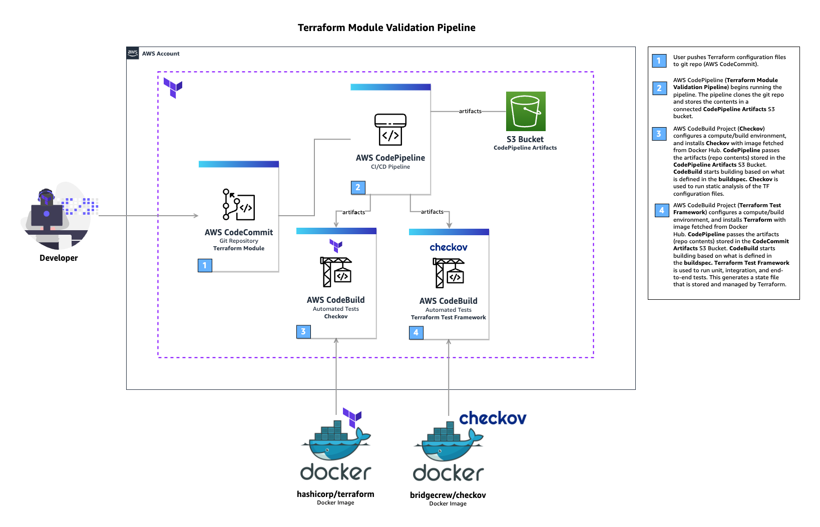
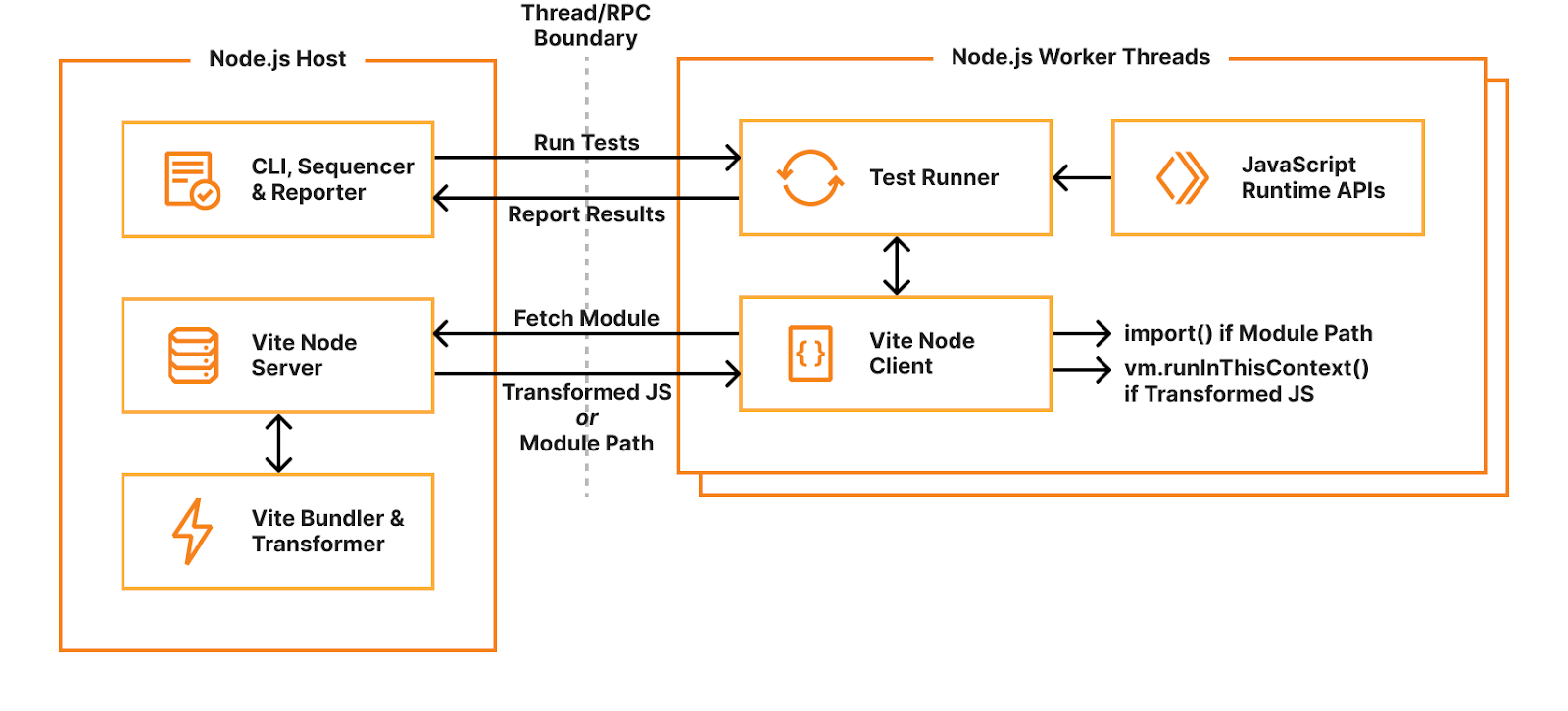
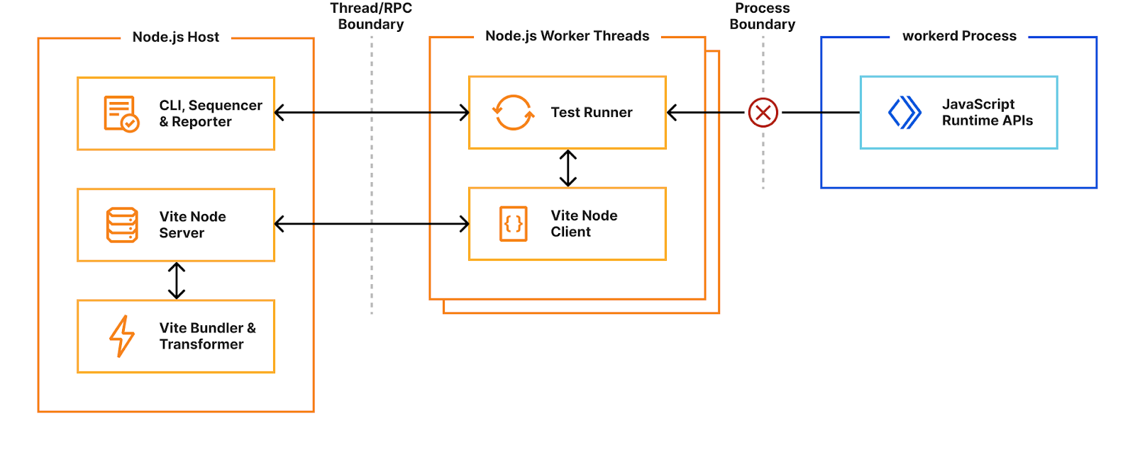
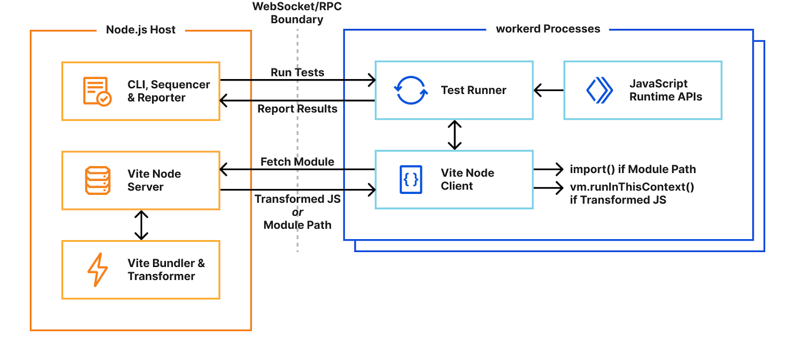
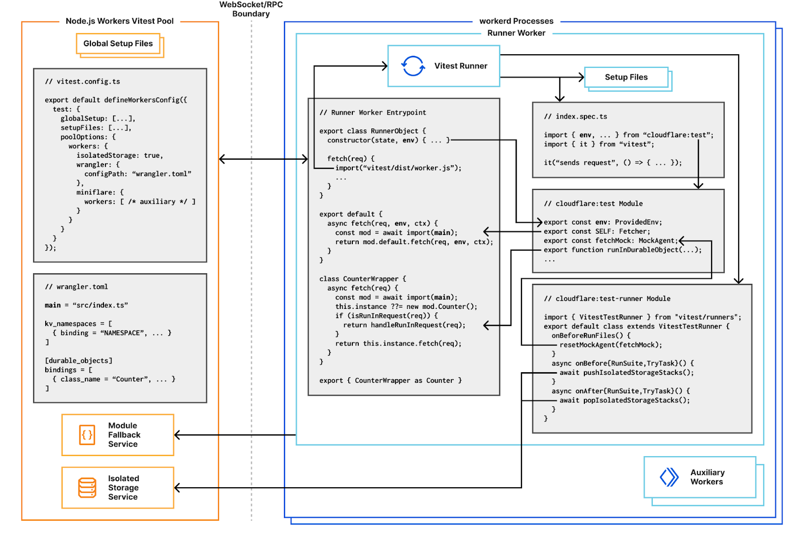
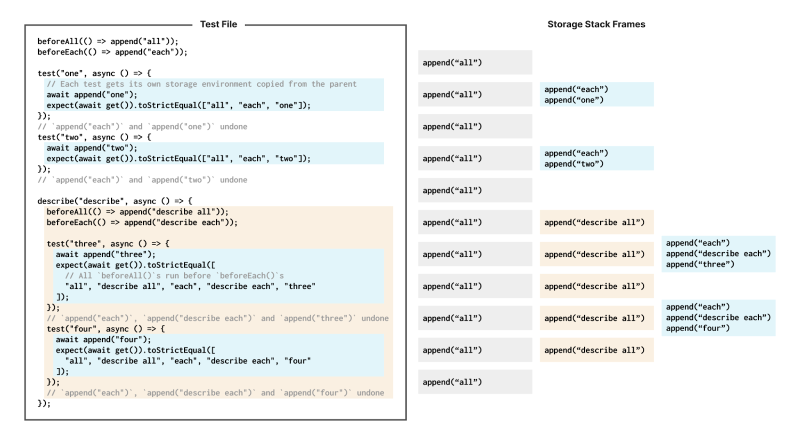
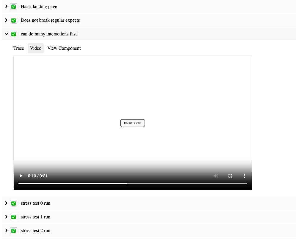


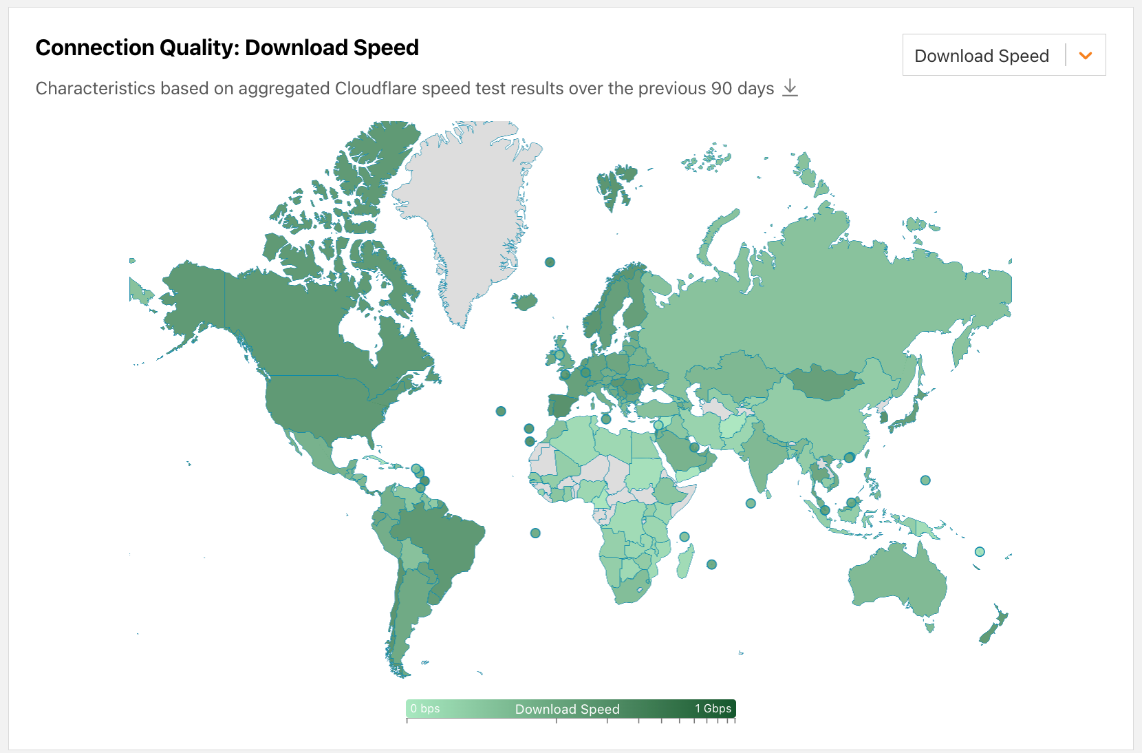
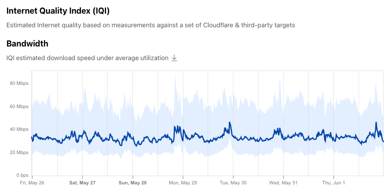
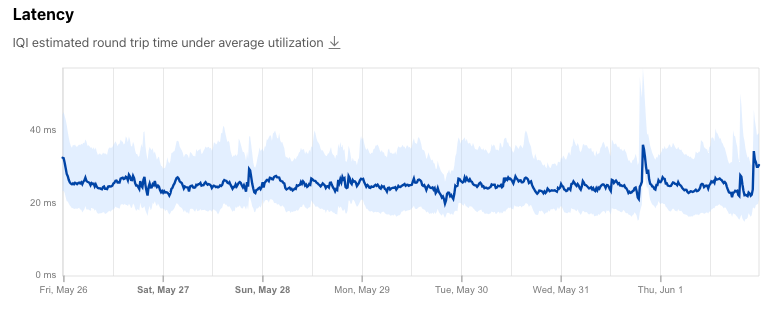

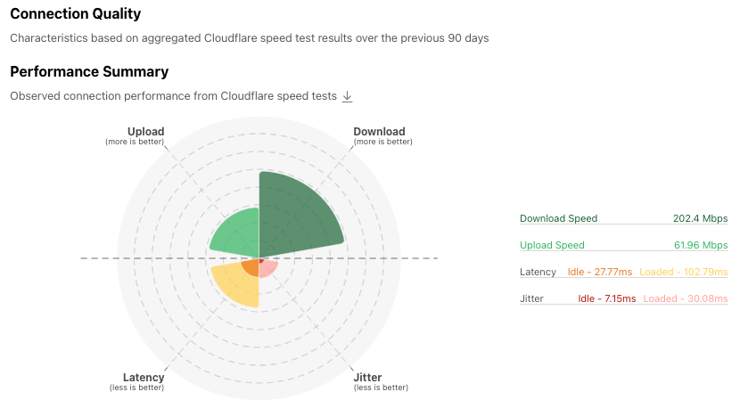

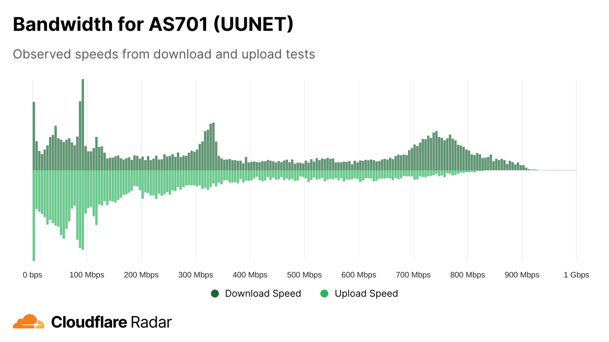

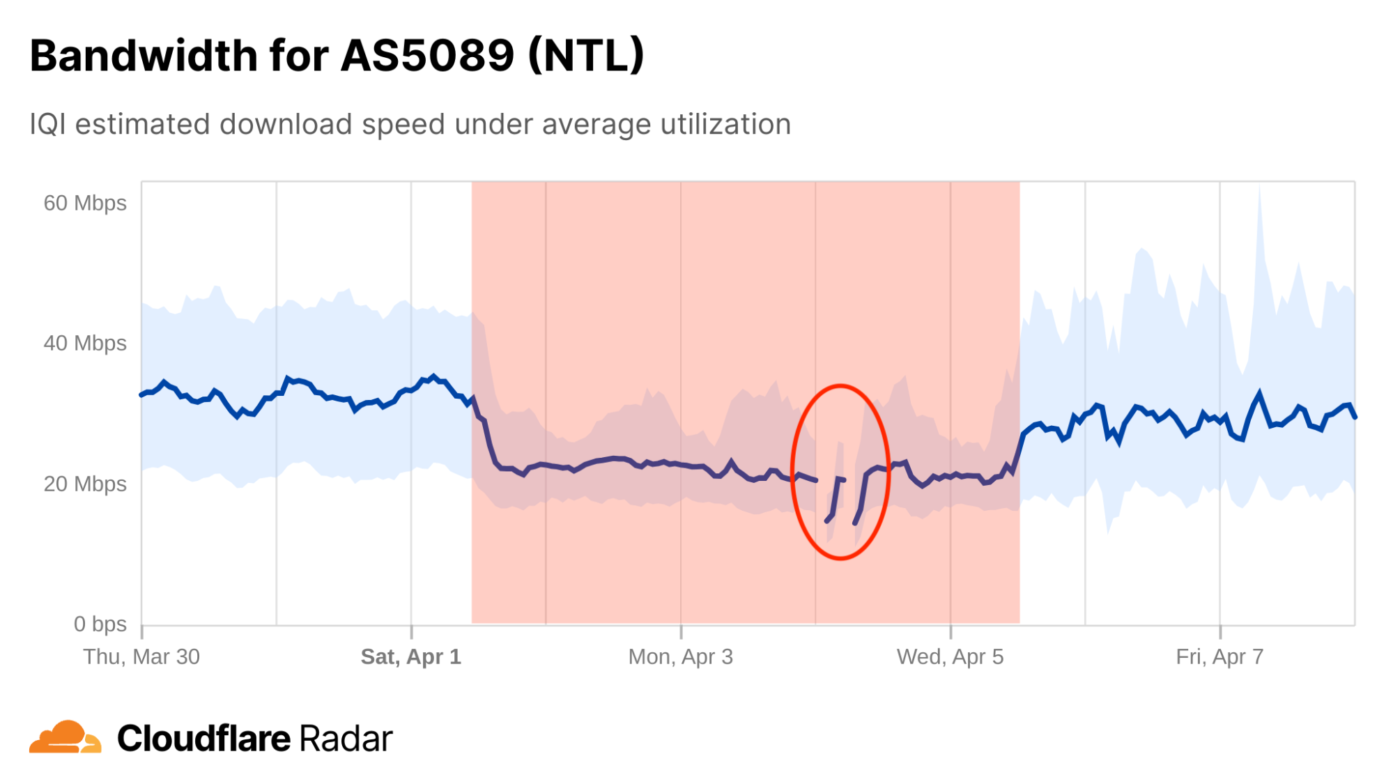

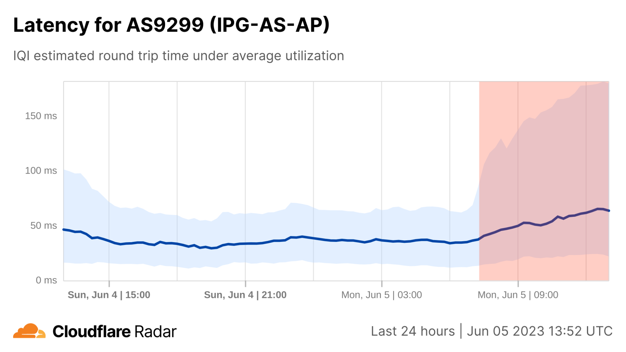
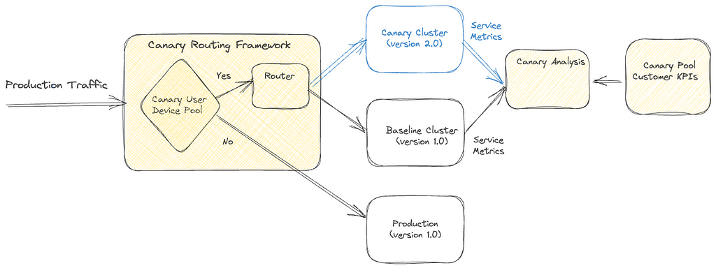
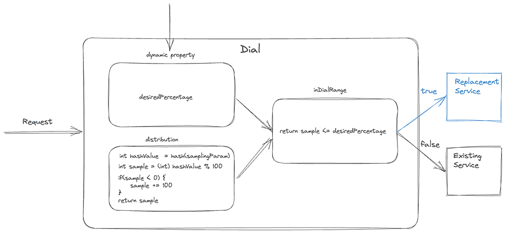


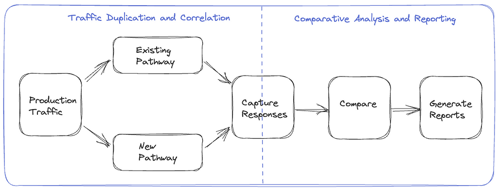


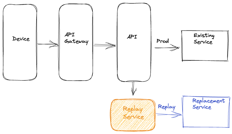

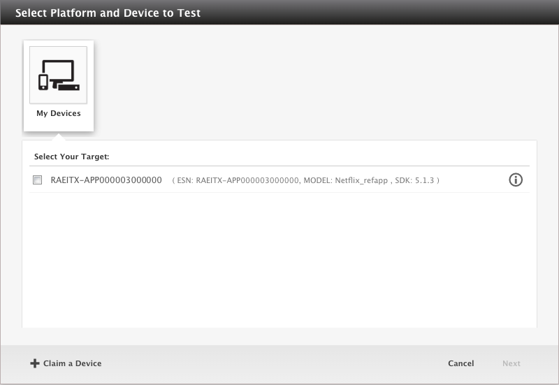

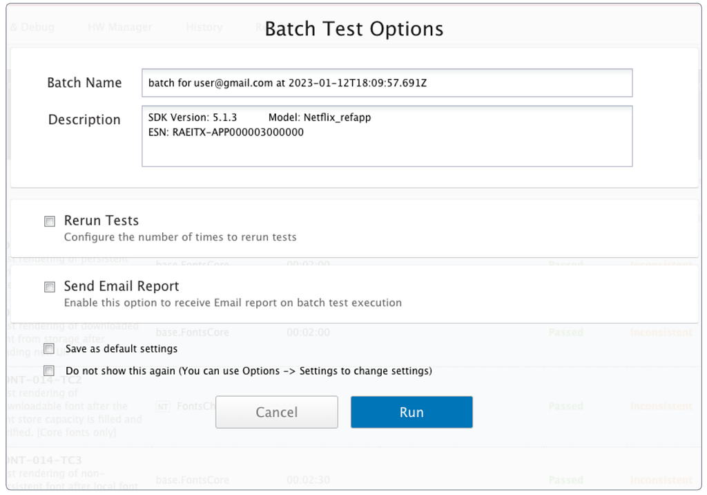
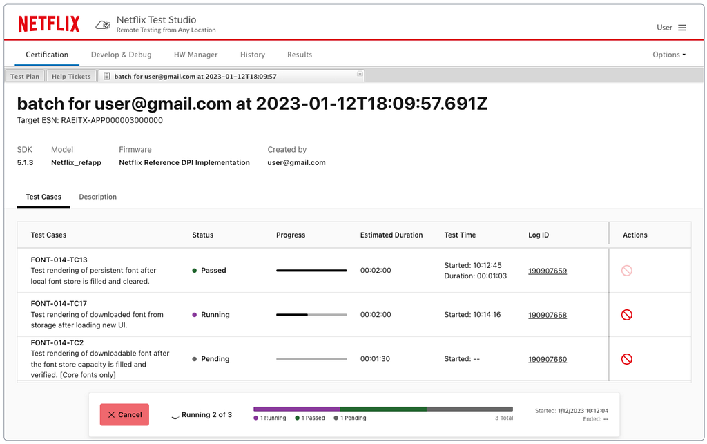
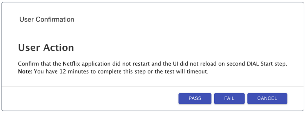
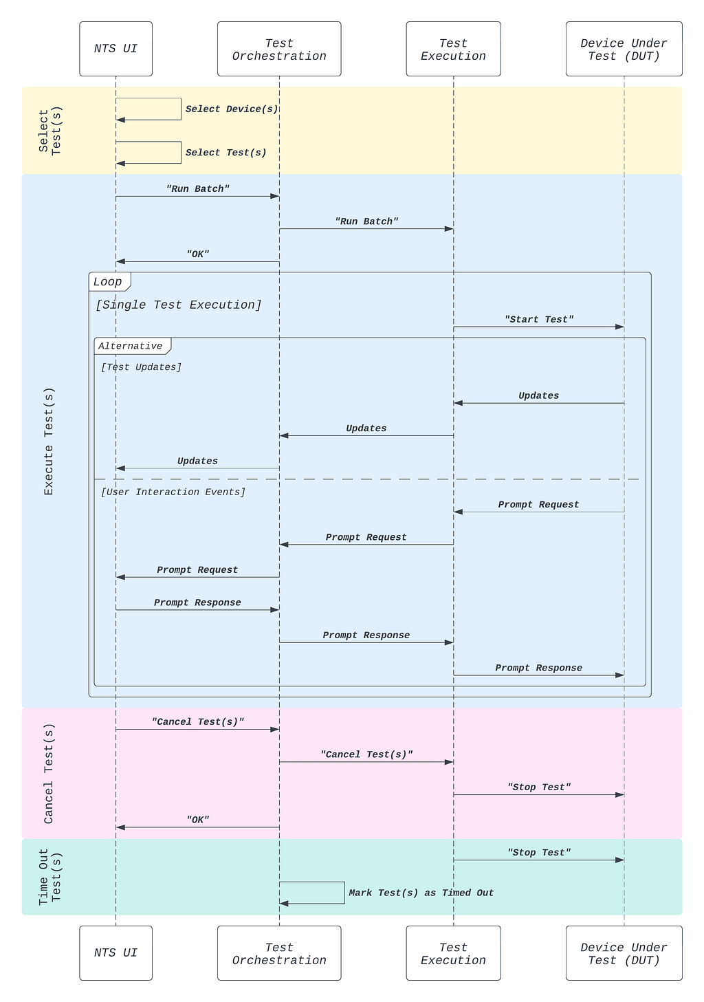
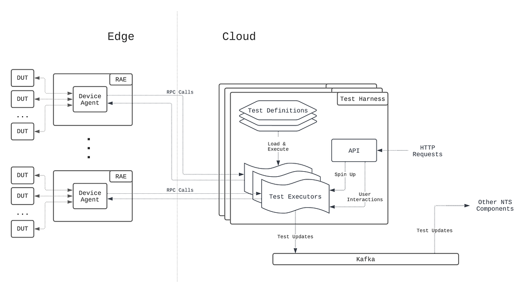


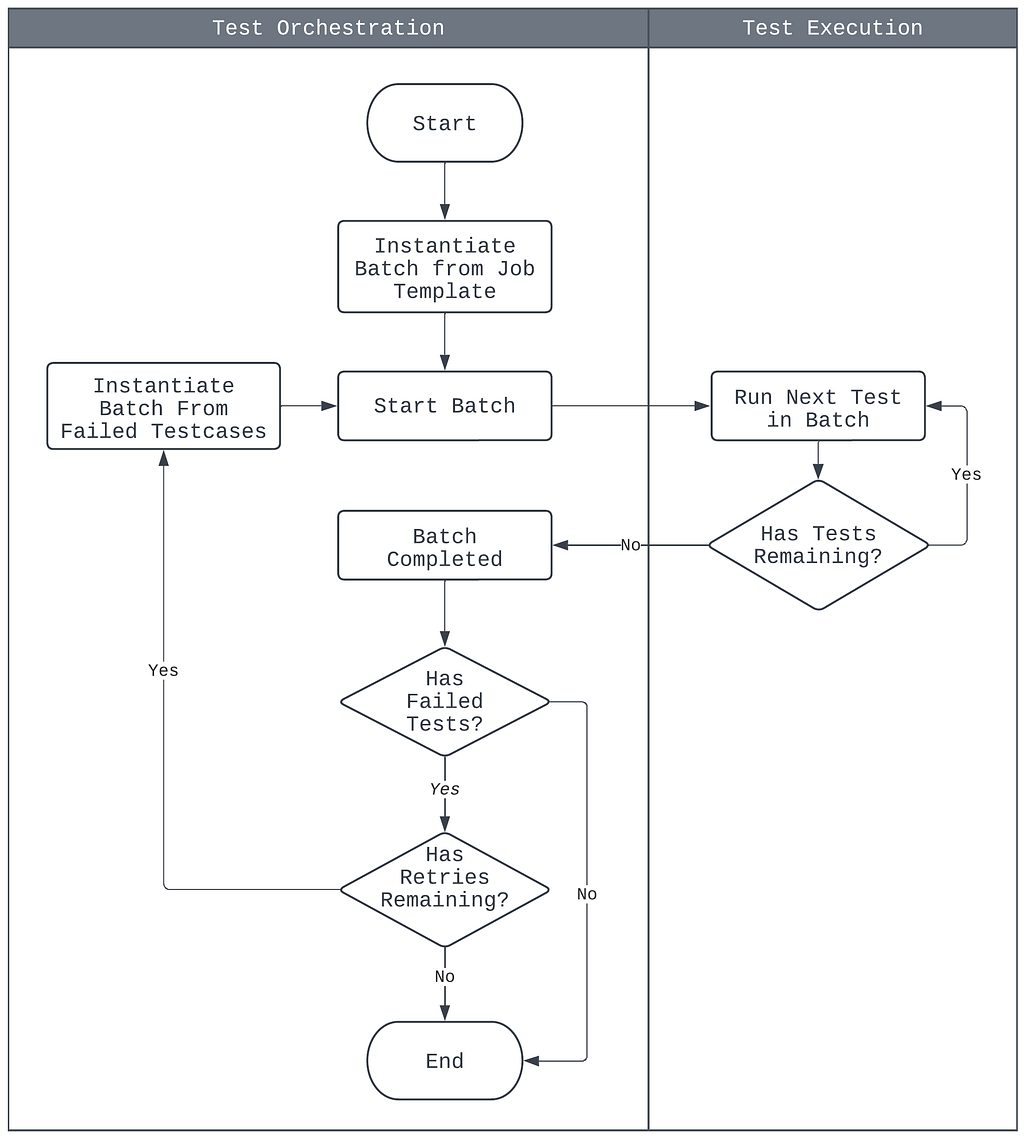


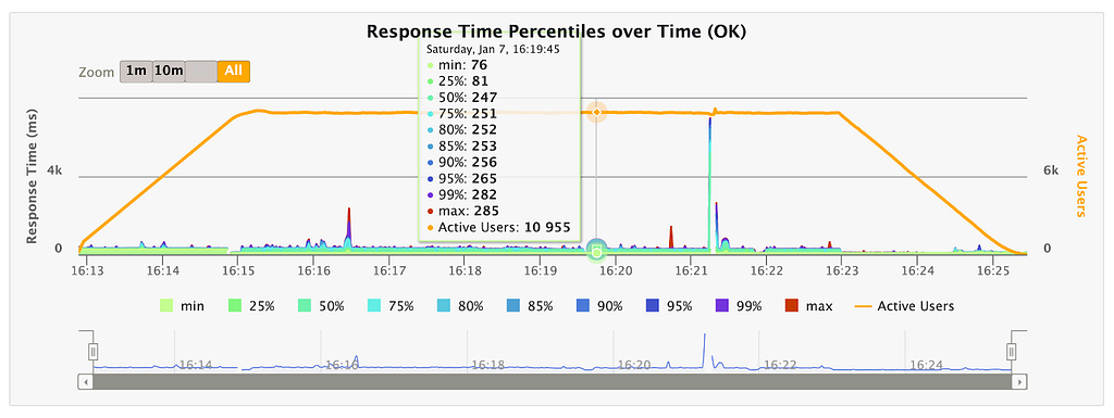


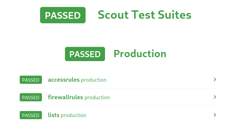
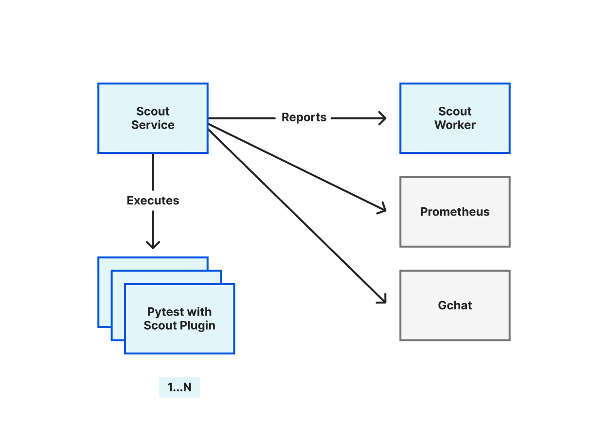
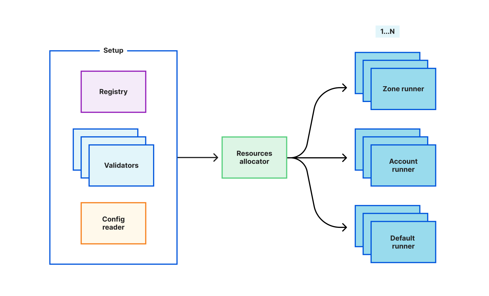
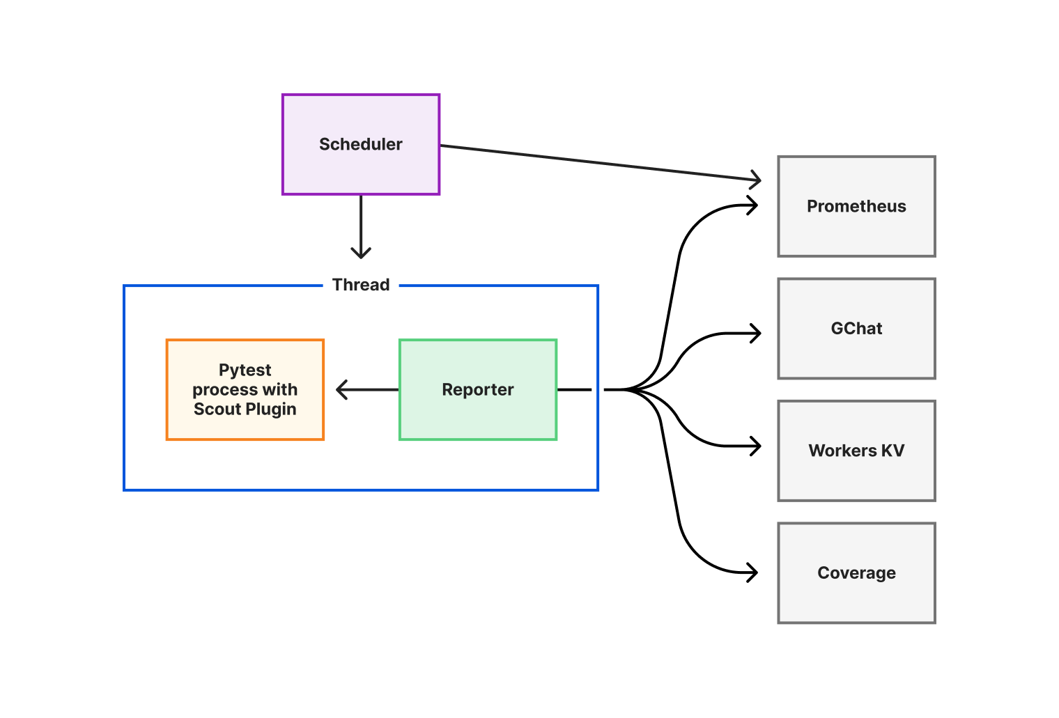
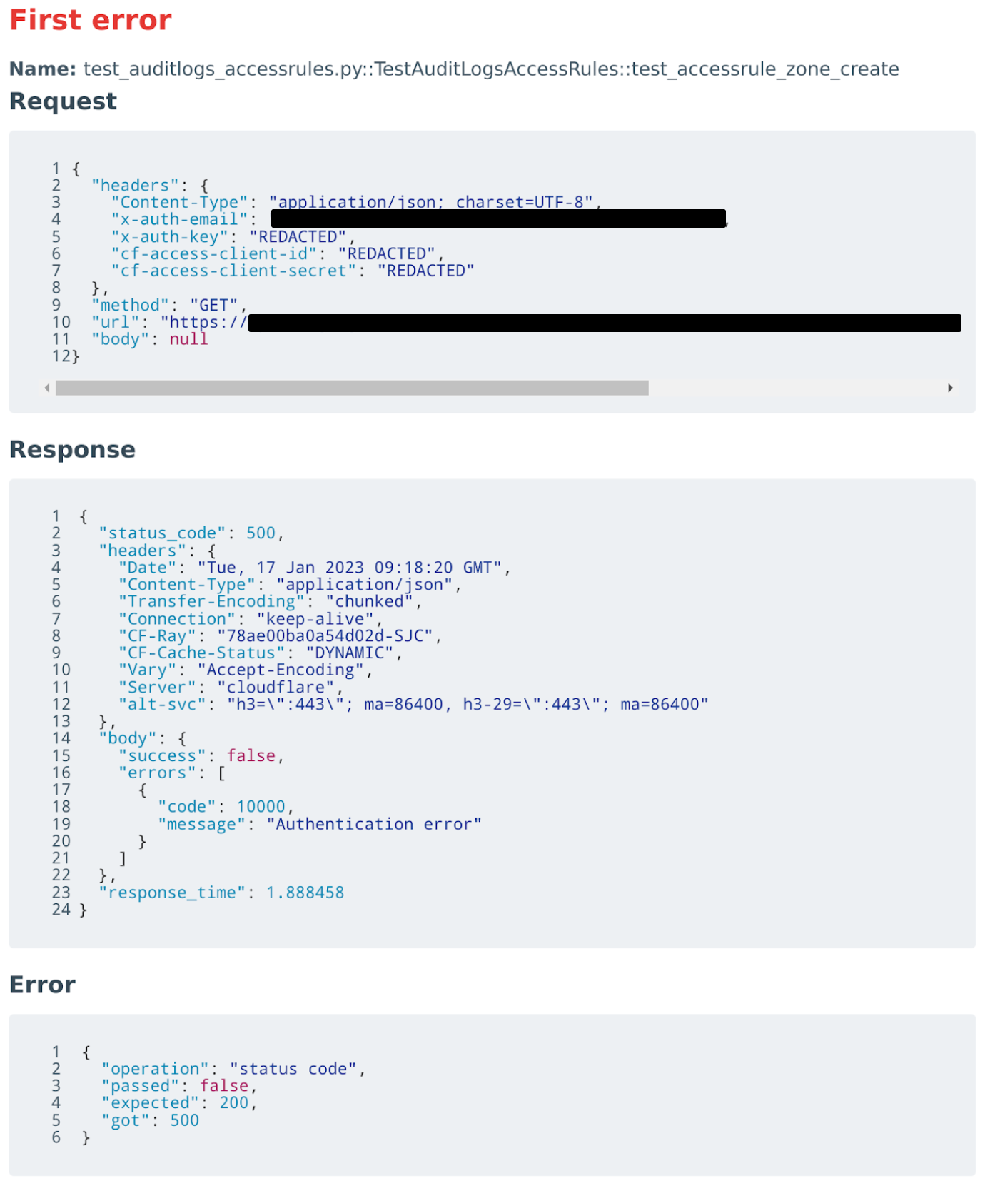


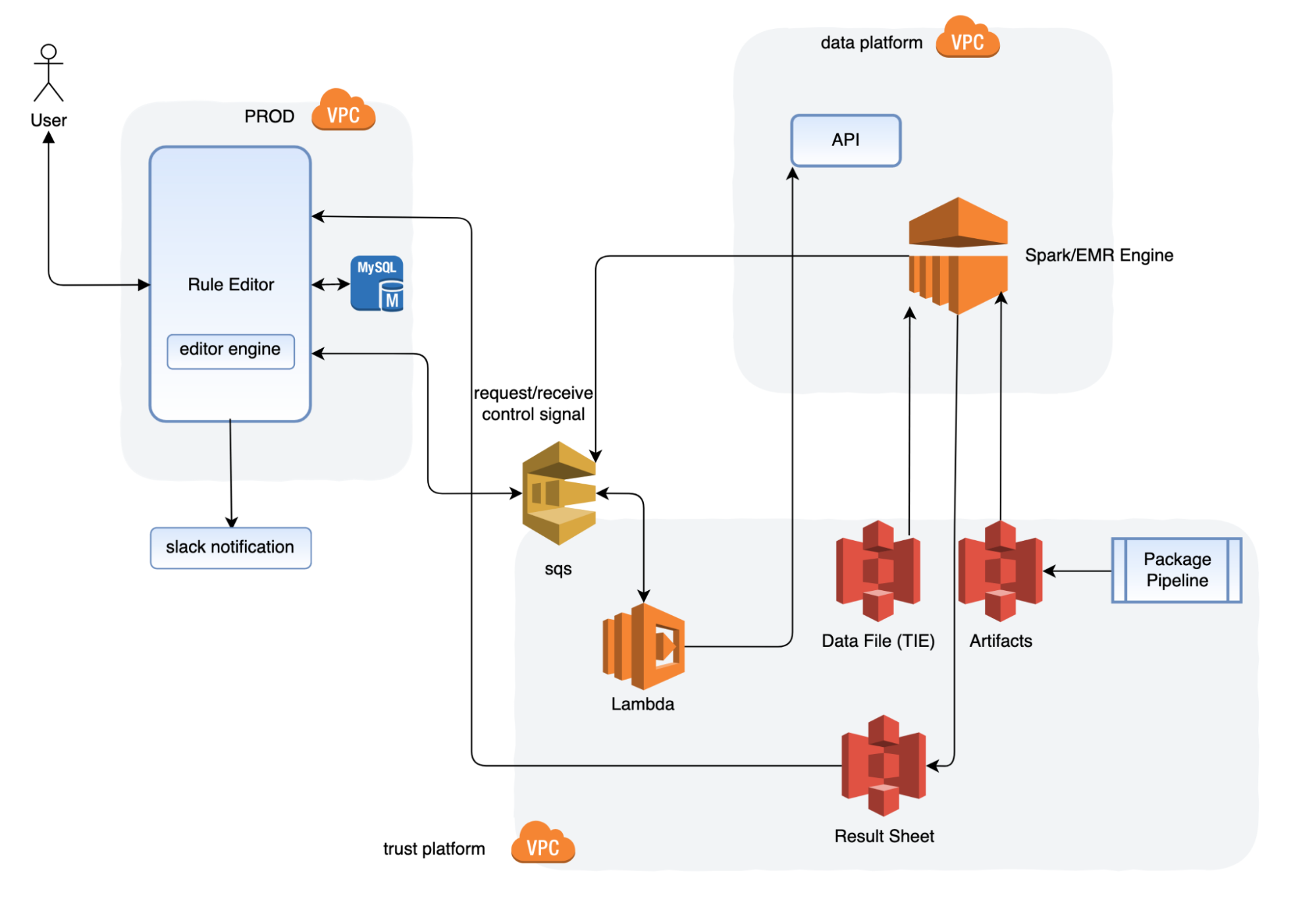

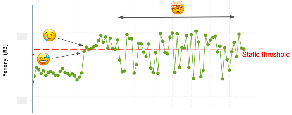


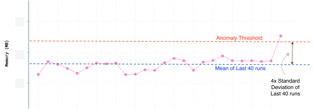
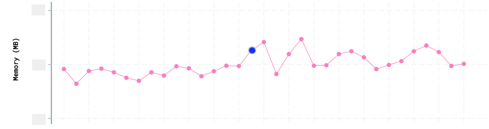
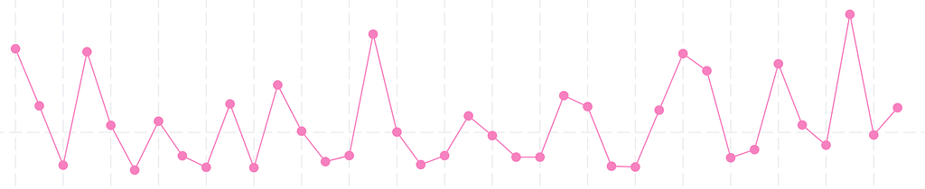
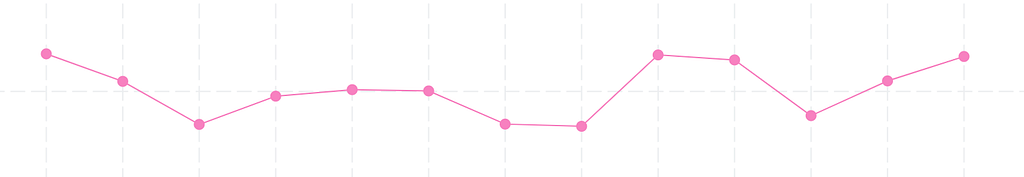
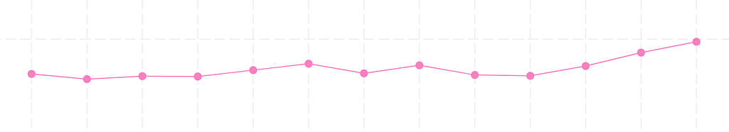


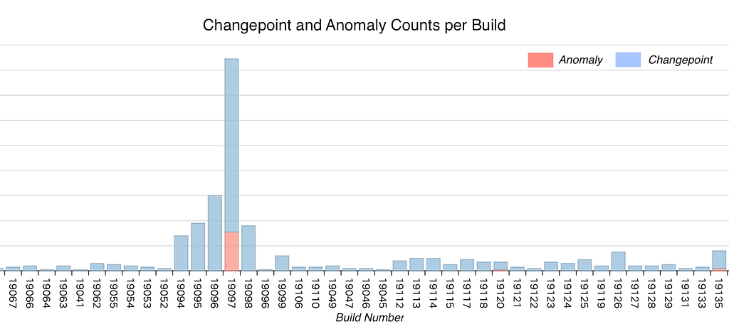
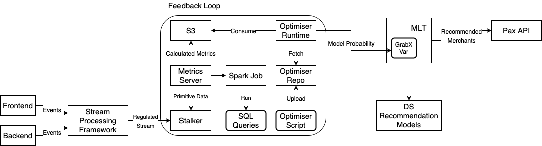

 .
. .
.